Session 1 — Introduction to Spatial Epidemiology
Spatial data · file formats · coordinate reference systems · John Snow · what spatial epidemiology is for · theory · MAUP, ecological fallacy, dependence and heterogeneity
This first session sets up the vocabulary for the whole course. It answers three questions: what makes data spatial, what spatial epidemiology is trying to achieve, and which problems are special to analysing health data by place.
The thread running through the session, and the rest of the course, is a sentence from the last slide: a map is often the beginning of the epidemiologic question, not the end. Seeing where disease is high leads to asking why it is high there, and then what can be done.
The second half introduces the methodological issues that come back in every later session: the modifiable areal unit problem (MAUP), the ecological fallacy, spatial dependence and spatial heterogeneity.
NoteSources and session
Slides: “session_1_v0-1.pdf” (Qinyun Lin, 6 October 2026, 13:15–15:00).
In-class activity: the story map on John Snow and the 1854 cholera outbreak (Center for Spatial Data Science, University of Chicago).
Lecture notes: the topics marked ✏️ were written down in class as important. The notes also record that the exam tests concepts, not programming.
TipBefore you start: three ideas from earlier courses
Rate vs count. A count (20 cases) depends on how many people there are. A rate or risk (20 cases per 1,000) divides by the population at risk, so areas of different size can be compared.
Confounding. An association between an exposure and an outcome can be produced by a third factor related to both. Place is often a stand-in for many such factors at once (income, pollution, access to care).
Independence in regression. Ordinary least squares (OLS) and the usual standard errors assume that, after accounting for the covariates, observations are independent. Session 1 introduces the reason why spatial data often break this assumption: nearby places resemble each other.
1.1 What is spatial data?
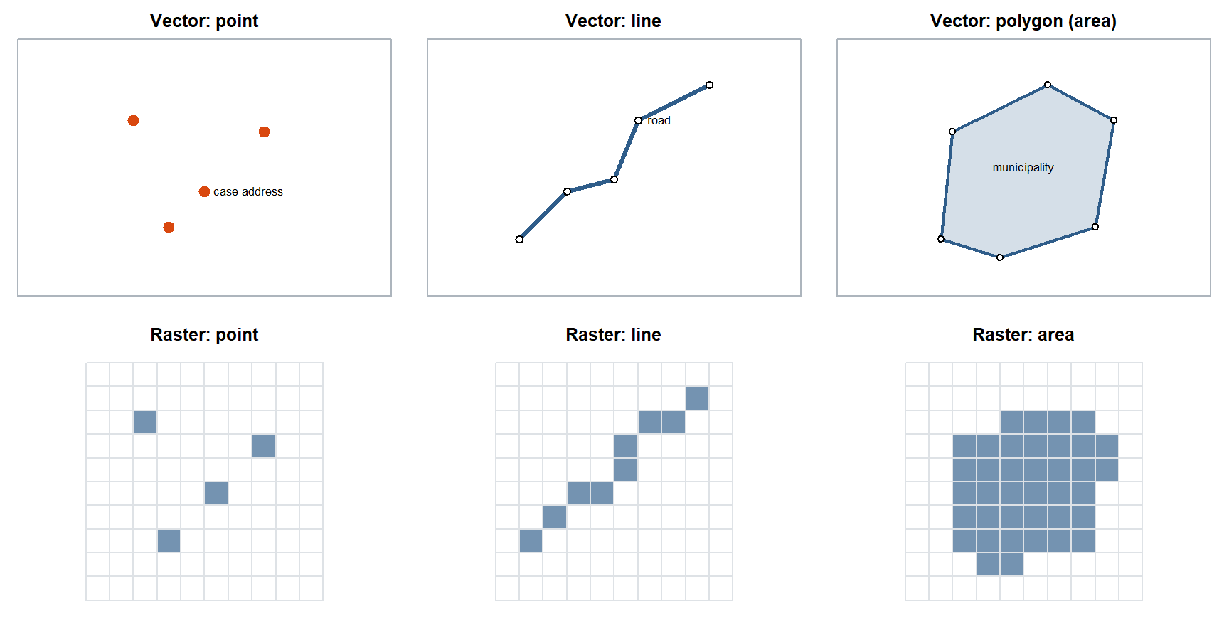
In short. Spatial data are ordinary data with a location attached. The location is stored either as exact shapes (vector: points, lines, polygons) or as a grid of cells (raster). Most of this course uses polygons: areas such as municipalities, each with a count or a rate.
Spatial data = information + location. The information (an attribute: a disease rate, an income, a pollution level) is tied to a place. The information may change with location; that is the point of studying it spatially. Very occasionally spatial data contain only location (a list of clinic coordinates), but without location the data are no longer spatial.
A spatial data file has two parts that belong together:
- the geometry: where each feature is (coordinates, or the outline of an area);
- the attribute table: one row per feature with its variables, like an ordinary data frame.
Two ways of representing space
| Model | How space is stored | Feature types | Typical health example |
|---|---|---|---|
| Vector | Exact coordinates of points and the vertices that join them | Point (one coordinate pair), line (connected points), polygon / area (closed line) | Case addresses (points), roads (lines), municipalities or DeSO areas (polygons) |
| Raster | A grid of equal cells; every cell holds a value | The same shapes, approximated by filled cells | Air-pollution surfaces, land cover, satellite temperature |
In the lecture notes, area = polygon. Most of this course works with areal (polygon) data: counts or rates aggregated to administrative areas.
Vector points for homes and a raster grid for pollution
Vector polygons for homes and vector lines for pollution
A raster grid for homes and vector points for pollution
Two raster grids at different cell sizes for both layers
A home address is a single coordinate pair, a vector point. A pollution surface measured on 1 km cells is a raster. Joining them means looking up the cell value at each point.
On the exam, be able to say: Spatial data = information + location. Vector data store points, lines and polygons as coordinates; raster data store values in a regular grid of cells.
1.2 Spatial file formats: CSV, shapefile, GeoJSON
In short. A spatial file has to carry three things: the shapes, the data table and the coordinate system. A shapefile splits them over at least four files that must stay together; GeoJSON keeps everything in one file; a CSV works only for points with coordinate columns.
| Format | What it is | Watch out for |
|---|---|---|
| CSV (or other text file) | An ordinary table. It is spatial only if it has coordinate columns (longitude, latitude) | Cannot store polygons in a practical way; the CRS is not recorded in the file |
| Shapefile | ESRI’s format. At least four files with the same name and different extensions | All files must sit in the same folder; if one is missing the layer breaks |
| GeoJSON | Open standard text format for points, lines and polygons with attributes | Can be large for detailed boundaries |
The four shapefile parts (as written down in class):
| Extension | Holds |
|---|---|
.shp |
The geometry: the shapes themselves |
.shx |
The index that lets software find each shape quickly |
.dbf |
The attribute table (one row per shape) |
.prj |
The projection: which coordinate reference system the coordinates are in |
“The .shp file is the shapefile, so I only need to send that.” The .shp holds the shapes but no attributes and no CRS. Without .dbf you lose the data columns, and without .prj the software does not know where on Earth the coordinates belong. Keep all parts together.
The .prj file, so the coordinate reference system is unknown
The .dbf file, so the attribute columns cannot be read
The .shx file, so the shapes cannot be indexed at all
A GeoJSON copy, which shapefiles need for their geometry
Shapes and attributes load fine (.shp, .shx, .dbf are there). What is missing is the projection information in .prj: without it, software cannot place or transform the coordinates correctly.
On the exam, be able to say: A shapefile has at least four parts in the same folder: .shp (geometry), .shx (index), .dbf (attribute table) and .prj (projection/CRS).
1.3 Coordinate reference systems and EPSG codes
In short. Coordinates mean nothing without a coordinate reference system (CRS): it says where on Earth the numbers point and how the round Earth was flattened. Put all layers in the same CRS before combining them, and use a CRS in metres for distances.
Think of it as: Currencies. “100” means nothing until you know whether it is kronor or euros, and you must convert before you add two amounts.
The Earth is round; a map is flat. A coordinate reference system (CRS) says how coordinates relate to places on the Earth’s surface, and for a projected CRS, which method was used to flatten (project) the surface onto two dimensions. Different projections give visibly different world maps: every projection distorts area, shape, distance or direction somehow.
CRSs are identified by EPSG codes (from the European Petroleum Survey Group): a standard number that pins down the datum, the coordinate system and the projection.
| EPSG:4326 (WGS 84) | EPSG:3006 (SWEREF 99 TM) | |
|---|---|---|
| Kind | Geographic (unprojected) | Projected |
| Coordinates | Longitude and latitude | Easting and northing |
| Units | Degrees | Metres |
| Typical use | GPS, web maps, data downloaded online | Swedish national spatial data |
| Distances and areas | Not directly: a degree of longitude shrinks towards the poles | Yes, Euclidean distance in metres is meaningful |
Two practical rules from the slides:
- Recognise 4326. Coordinates like
41.784766, -87.609299(small numbers with many decimals, within ±90 and ±180) are almost certainly longitude/latitude in EPSG:4326. Try that first. - Transform before you join. When you combine layers, put everything in the same CRS first. Layers in different CRSs will not line up, and spatial joins or distances will be wrong.
For distance or area calculations, transform to a suitable projected CRS (in Sweden, SWEREF 99 TM). This returns in Session 2: Euclidean distance between points is only meaningful for projected coordinates.
Transform the points to a projected CRS in metres, such as SWEREF 99 TM
Use a 5-degree distance band, because the coordinates are in degrees
Nothing, since Euclidean distance works the same in any CRS
Convert the shapefile to GeoJSON, which stores distances in metres
In EPSG:4326, coordinates are in degrees, and one degree is not a fixed number of metres. A 5 km threshold needs projected coordinates in metres (or great-circle distances). File format does not change the CRS.
On the exam, be able to say: A CRS defines how coordinates relate to the Earth’s surface; EPSG codes identify it. EPSG:4326 (WGS 84) is in degrees; projected systems such as SWEREF 99 TM (EPSG:3006) are in metres and are needed for distances and areas. Layers must share a CRS before they are joined.
1.4 Geocoding and Swedish small areas (DeSO)
In short. Geocoding turns an address into coordinates. Health data are usually reported for administrative areas; in Sweden the smallest standard unit is DeSO.
Geocoding turns an address into coordinates (longitude and latitude), so that individuals can be placed on a map or linked to the area they live in. Geocoding can fail or be wrong (missing or misspelled addresses, rural addresses placed at a postcode centroid). Such errors are rarely random: they are more common in some kinds of areas, which can bias a spatial analysis (see 1.13).
Most health data are reported for administrative areas: province, county, postcode, census tract. In Sweden the smallest standard statistical unit is DeSO (demografiska statistikområden, demographic statistical areas), designed by Statistics Sweden to have roughly 700 to 2,700 inhabitants each, so that statistics can be published at fine scale without identifying people. The lecture notes record DeSO as the smallest area in Sweden used in practice.
Why the choice of unit matters is the subject of 1.10 Scale and MAUP.
On the exam, be able to say: Geocoding converts addresses to longitude/latitude; failures are often concentrated in some areas, so they are not random. DeSO are Sweden’s small statistical areas of roughly 700–2,700 inhabitants.
1.5 John Snow and the 1854 cholera outbreak
In short. In London in 1854, John Snow mapped cholera deaths and water pumps. Deaths clustered around one pump, and comparing households with different water supplies supported his idea that cholera spreads through water, not “bad air”.
The in-class activity: read the story map (about 15 minutes) and answer three questions.
| Question | Answer |
|---|---|
| Research question | What causes cholera, and why did so many people in one part of Soho, London, die in a few days in 1854? |
| Competing hypotheses | Miasma: disease spreads through “bad air” from rotting matter (the dominant view). Waterborne: cholera is transmitted through contaminated water (Snow’s hypothesis) |
| Spatial data used | The locations of cholera deaths (point data, stacked as bars at each house) and the locations of public water pumps on a street map. Snow also compared deaths by which water company supplied a household |
The map showed deaths clustered around the Broad Street pump. Exceptions were informative: workers at a brewery with its own water supply were largely spared, while some deaths far away were in people who preferred to fetch water from Broad Street. The pump handle was removed.
Classifying Snow’s work with the describe–analyze–intervene framework (1.7): mapping the deaths describes; testing the water hypothesis against miasma (including the comparison of water companies) analyzes; removing the pump handle is an intervention. One study can move across all three goals, which is exactly what modern spatial epidemiology rarely does.
“Snow’s map proved the cause.” The map alone shows clustering around a pump, which miasma could also explain (bad air near the pump). What made the argument strong was theory (a waterborne mechanism), informative exceptions, and a comparison between households with different water supply. A map starts the question; the comparison answers it.
On the exam, be able to say: Research question: what caused the outbreak and how cholera spreads. Competing hypotheses: miasma (bad air) vs contaminated water. Data: death locations (points), pump locations and water supply by household. Snow described, analysed and intervened (the pump handle).
1.6 Definitions of spatial epidemiology
In short. Spatial epidemiology studies how disease varies between places, and why. The newer, broader definition adds that the aim is also to act: to inform interventions that improve health.
Three definitions from the slides, from narrow to broad:
| Source | Definition (key words) |
|---|---|
| Elliott & Wartenberg (2004) | “the description and analysis of geographic variations in disease with respect to demographic, environmental, behavioral, socioeconomic, genetic, and infectious risk factors” |
| Lawson (2018) | uses geographic location to understand the distribution of health outcomes and their determinants, considering how location influences the interaction of risk factors |
| Morrison et al. (2024), broader | applies theory and methods from epidemiology, geography and statistics to describe spatial distributions, analyze possible causes, inform intervention, and improve health |
The lecture notes record the first definition: geographic variations in disease with respect to demographic and other risk factors. Be able to reproduce one definition in your own words and say what the broader one adds: an explicit aim to explain and to intervene, not just to map.
On the exam, be able to say: Spatial epidemiology is the description and analysis of geographic variation in disease with respect to demographic, environmental, behavioural, socioeconomic, genetic and infectious risk factors. Morrison et al. broaden it to describe, analyse and intervene.
1.7 Describe → analyze → intervene (Morrison et al. 2024)
In short. A study can describe (where is disease?), analyse (why there?) or intervene (what can we change?). A large review found many descriptive and analytic studies but no intervention studies.
Think of it as: A doctor who is excellent at diagnosis and at explaining the illness, but never tests a treatment.
Morrison et al. (2024, Epidemiology 35(4):542–555) reviewed the spatial epidemiology literature and asked whether the field is aligned with the broader goals of epidemiology.
flowchart LR
  D["DESCRIBE<br/>Where is health distributed?<br/>(disease mapping, cluster detection,<br/>surveillance, resource allocation)"] --> A["ANALYZE<br/>Why might the pattern occur?<br/>(place-based determinants,<br/>exposure–outcome relationships,<br/>mechanisms, inequalities)"]
  A --> I["INTERVENE<br/>What can we change?<br/>(target interventions, evaluate<br/>place-based policies,<br/>change environments)"]
What the review found among 482 papers:
| Type | Number |
|---|---|
| Descriptive | 122 |
| Analytic | 167 |
| Intervention | 0 |
| Reviews | 76 |
| Demonstrations of methods | 117 |
Zero intervention studies. The field is good at mapping patterns and developing methods, but mainly describes and explains; it rarely evaluates what works. The slides’ re-orientation: spatial statistical methods are tools, not the endpoint. The question is not only “Where are the clusters?” but “Why are they there, and what can we do about them?”
From where to why requires more than a map: pattern → theory → analysis. Theory tells you which spatial units, exposures, pathways, confounders and mechanisms are meaningful.
On the exam, be able to say: Morrison et al. (2024) classified 482 papers: 122 descriptive, 167 analytic, 0 intervention. Spatial methods are tools, not the endpoint: the field should move from where to why to what can be done.
1.8 Why place matters for health
In short. Where people live shapes what they are exposed to (air, noise, food) and what they can reach (care, parks, schools). That is why place itself is studied as a determinant of health.
Physical and social environments produce health disparities. Examples from the slides:
- longer distance to mammography facilities → later breast cancer diagnosis (Nattinger 2001; note: the paper itself studies distance to a radiotherapy facility and the choice of breast cancer surgery);
- pedestrian-friendly environments → lower obesity (Gordon-Larsen 2006);
- living along major traffic corridors → cardiovascular disease (McEntee 2008; note: the paper itself studies diesel particulate matter, lung cancer and asthma along traffic corridors).
Three frameworks that put place inside epidemiology:
| Framework | Core idea |
|---|---|
| Social determinants of health (WHO 2010) | The conditions in which people are born, grow, live, work and age, including neighbourhood and physical environment and access to healthcare, shape health |
| Eco-epidemiology (Schwartz et al. 1999) | Individuals are interdependent and connected to the biological, physical, social and historical contexts they live in |
| Multiple exposures over the life span (Buck Louis & Sundaram 2012) | Measure many environmental exposures at different times in life, not one exposure at one time |
The common message: place stands for context: access to food, care, education, green space and clean air.
On the exam, be able to say: Physical and social environments produce health disparities (for example distance to care, walkability, traffic exposure). Frameworks: social determinants of health, eco-epidemiology, multiple exposures across the life span.
1.9 Theoretical frameworks: social-ecological model and life course
In short. Two ways to organise the causes of health. The social-ecological model places the individual inside nested levels (relationships, organisations, community). The life-course model describes five steps through which social position becomes unequal health. Spatial data fit at the neighbourhood level.
Both frameworks were written down in class.
Social-ecological model (Bronfenbrenner 1994; Dahlberg & Krug 2002). Health is shaped by nested levels:
| Level | Example from the slide (stigma around opioid use disorder) |
|---|---|
| Individual | Age, race/ethnicity, education |
| Interpersonal | Friends’ or family members’ experience with the disorder |
| Organizational | Workplaces, clinics, schools |
| Community / neighbourhood | Spatial access to treatment (medication for opioid use disorder) |
Spatial data enter at the outer level: the neighbourhood and what is reachable from it.
Life-course perspective: five mechanisms behind social inequality in health (Diderichsen et al. 2001):
| Mechanism | Where spatial data can help | |
|---|---|---|
| I | Social stratification: people end up in different social positions | Residential segregation by income |
| II | Differential exposure: lower positions meet more causes of illness | Pollution, noise, unhealthy food environments by area |
| III | Differential vulnerability: the same exposure harms some groups more | Area deprivation modifying the effect of heat |
| IV | Differential disease consequences: illness leads to worse outcomes for some | Distance to care, late diagnosis |
| V | Consequences for the individual and society: illness feeds back into social position | Job loss concentrated in some areas |
The in-class discussion question was where spatial data and spatial epidemiology may be useful, and how. A good answer links one mechanism to one spatial measure, as in the right-hand column.
On the exam, be able to say: Social-ecological model: individual, interpersonal, organisational and community levels. Diderichsen’s five mechanisms: social stratification, differential exposure, differential vulnerability, differential consequences, and consequences for the individual and society.
1.10 Scale and the modifiable areal unit problem (MAUP)
In short. Results from area data depend on which areas you use. Make the areas bigger, or draw the borders differently, and the map and the statistics can change, even though the people are the same.
Think of it as: Average grades by class, by school or by municipality: each level tells a different story about the same pupils.
Health data are usually aggregated to administrative zones (province, county, postcode, census tract, DeSO). These units:
- are often irregular and arbitrary, drawn for administration, not for health;
- can change over time (inconsistent geography), which makes trends hard to follow.
The modifiable areal unit problem (MAUP) (Openshaw 1984): changing the spatial units can lead to different statistical results and interpretations, even when the underlying individual data are the same. The lecture notes put it as: if we change scale (new areas are under investigation), the interpretation will change.
MAUP has two parts:
| Effect | What changes | Example |
|---|---|---|
| Scale effect | The size of the units (DeSO → municipality → county) | A correlation between deprivation and mortality gets stronger as units get larger, because aggregation averages out individual noise |
| Zoning effect | Where the boundaries are drawn, at the same size | Two ways of drawing 20 equal-sized districts give different cluster maps |
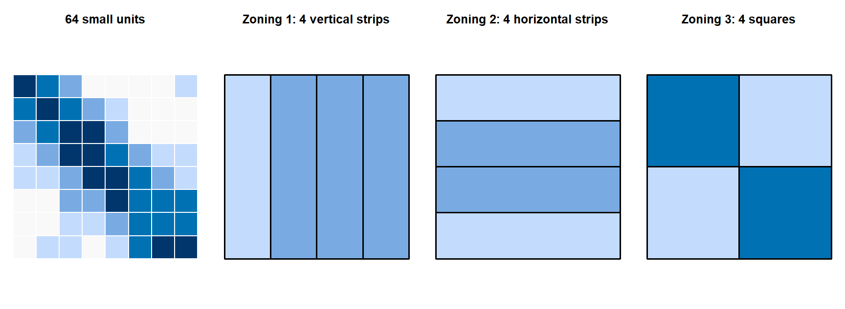
A partial remedy from the slides: a regular hexagon grid (all units the same size and shape), but health data are rarely available on such grids.
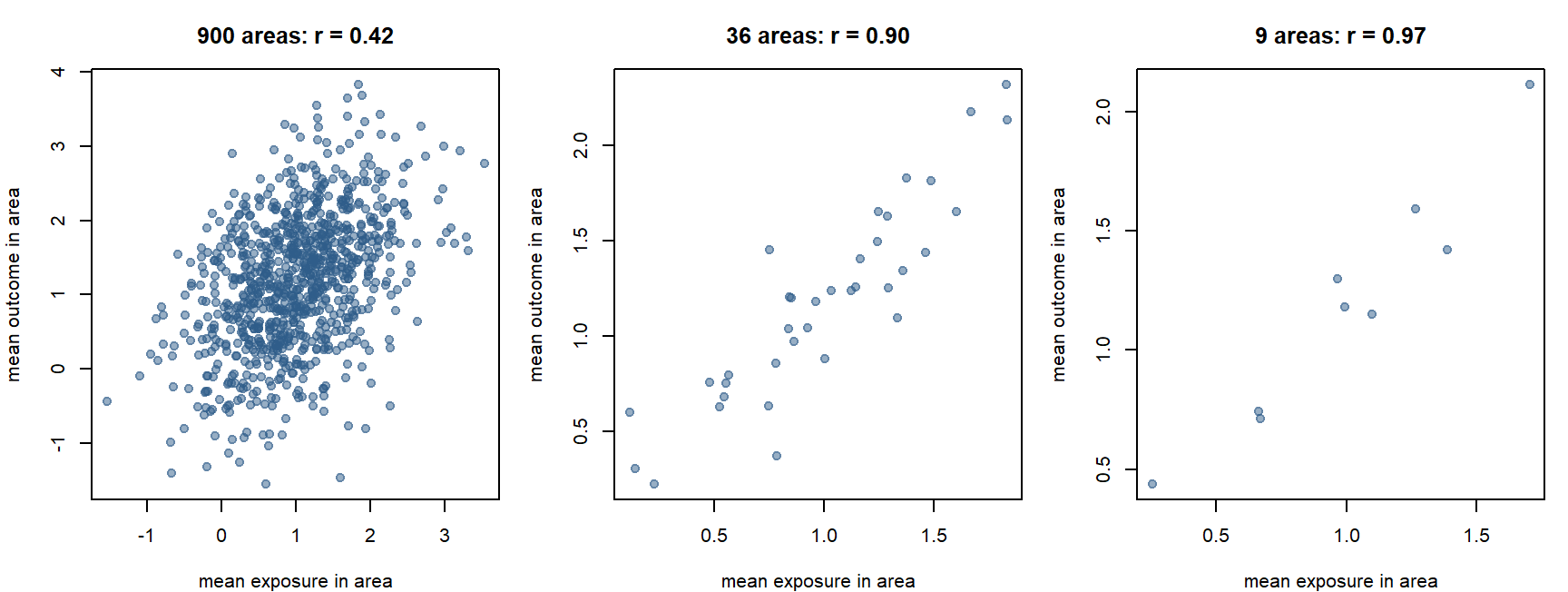
The individual-level correlation in this simulation is about 0.25. None of the area-level correlations is “the” answer: each describes associations between areas at that scale.
TipWhen to use this idea
Whenever results come from aggregated data: say which unit was used, ask whether conclusions hold at another scale, and prefer units that make sense for the mechanism (a health-care catchment for access to care, a smaller unit for air pollution).
On the exam, be able to say: MAUP: changing the spatial units (scale effect: their size; zoning effect: where the borders go) can change results and interpretations even though the underlying data are the same.
1.11 The ecological fallacy
In short. A pattern between areas does not have to hold for the individuals in them.
Think of it as: A neighbourhood with high income and many votes for one party does not prove that the rich residents voted for that party.
Ecological fallacy (Robinson 1950): drawing incorrect inferences about individuals from group-level data.
Example from the slides: a region has a high crime rate, so one concludes that an individual from that region is likely to commit a crime. The aggregate does not describe individual characteristics or behaviour.
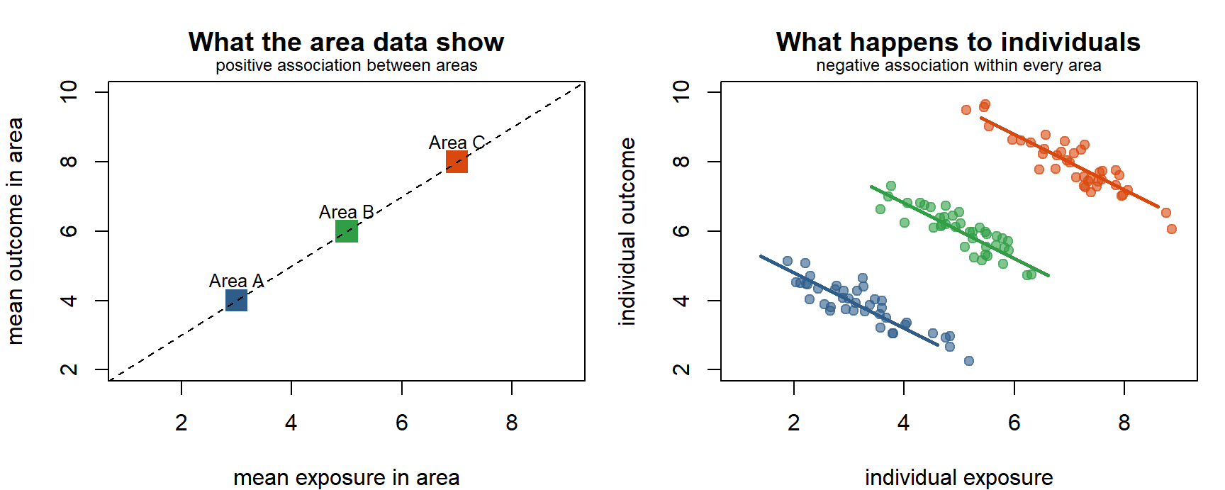
MAUP vs ecological fallacy. Both come from aggregation, but they ask different things:
| MAUP | Ecological fallacy | |
|---|---|---|
| The problem | Area-level results depend on how the areas are drawn | Area-level results are wrongly applied to individuals |
| Level of the conclusion | Stays at area level | Jumps from area to individual level |
| Question it raises | Would I see the same pattern with other units? | Does this association hold for people? |
The ecological fallacy: an area association is applied to individuals
The modifiable areal unit problem: the boundaries were drawn badly
Spatial heterogeneity: the association differs between regions
Geocoding error: outlets were placed in the wrong municipality
The data are at municipality level. Whether the individuals with diabetes ate fast food is not observed; inferring it is the ecological fallacy. MAUP would be the issue if the conclusion were about municipalities but changed with other boundaries.
On the exam, be able to say: The ecological fallacy is drawing conclusions about individuals from group-level data. It differs from the MAUP, which is about area-level results changing with the choice of areas.
1.12 Spatial dependence and spatial heterogeneity
In short. Dependence: neighbours tend to be alike. Heterogeneity: the rules themselves change from place to place.
Think of it as: Dependence: houses on the same street have similar prices. Heterogeneity: an extra room adds more to the price in Stockholm than in a small town.
These are the two properties that make spatial data special, and they motivate every method in the rest of the course.
Spatial dependence. Tobler’s first law of geography: “things closer together are more similar than things further apart”. Observations near one another may be more similar (or otherwise related) than observations far apart. Example: expensive and cheap neighbourhoods cluster because of socio-spatial processes. Dependence usually holds within some distance; beyond it, observations behave as independent.
Global measures summarise dependence in one number:
| Measure | Reading |
|---|---|
| Moran’s I ≈ 0 | Little or no global spatial autocorrelation |
| Moran’s I > 0 | Similar values tend to occur near one another (clustering) |
| Moran’s I < 0 | Dissimilar values tend to occur near one another (checkerboard) |
| Geary’s C | An alternative global measure (built on squared differences between neighbours) |
Both can be tested for statistical significance; Session 2 shows how.
Spatial heterogeneity. Processes and relationships differ by location, so one model applied everywhere can miss local patterns. Example: the relationship between income and housing prices differs between urban and rural areas. It shows up as regression coefficients that vary across regions, or as spatially structured random effects (Session 4).
| Spatial dependence | Spatial heterogeneity | |
|---|---|---|
| About | Similarity between nearby values | Differences in processes or relationships across space |
| Question | Are neighbours alike? | Is the same model valid everywhere? |
| Methods in this course | Moran’s I, LISA (S2); spatial lag and error models (S3); structured random effects (S4) | Mentioned; GWR and similar models are outside the course (S3) |
Spatial heterogeneity: the relationship differs by location
Spatial dependence: neighbouring admission counts are similar
The ecological fallacy: area data are applied to individuals
The MAUP: the result depends on the boundaries used
A relationship (temperature → admissions) that changes across space is heterogeneity. Dependence would be about values in neighbouring areas resembling each other, which can be present at the same time but is a different property.
On the exam, be able to say: Spatial dependence (Tobler’s first law): nearby observations are more similar than distant ones; measured by Moran’s I. Spatial heterogeneity: processes or relationships differ by location, so one global model can miss local patterns.
1.13 Other issues: reporting, geocoding, boundaries, sparse counts
In short. A map can show the data system instead of the disease: missed reports, failed geocoding, changing borders and tiny populations all create patterns that are not real.
The slides list four further problems. Each is a form of bias in spatial data (the course syllabus asks you to reflect on bias from aggregation, measurement and missing data):
| Issue | Why it can bias a map or model |
|---|---|
| Incomplete or geographically varying reporting | If some regions report less completely, they look healthier than they are. The map shows the reporting system, not the disease |
| Geocoding failure or error | Failed addresses are dropped or misplaced; failures are often concentrated in rural or new areas (missing data that are not missing at random) |
| Boundary changes over time | Areas merge or split, so rates before and after are not comparable (inconsistent geography) |
| Differences in population size / sparse counts | Small areas give unstable rates: extreme values may be chance, not risk. Session 2 (smoothing) and Session 4 (Bayesian disease mapping) deal with this |
On the exam, be able to say: Sources of bias: geographically varying reporting, geocoding failures (missing not at random), boundary changes over time, and unstable rates from small populations.
1.14 Tools: GIS, R and GeoDa
In short. GIS is the toolbox for storing, linking, mapping and analysing data by location. The course uses R and GeoDa.
GIS (geographic information systems) and related geospatial methods made spatial epidemiology practical: storing, linking, mapping and analysing data by location. Researchers use R, Stata, ArcGIS, GeoDa, Python and others.
In STA530:
- R: the main environment for spatial data analysis and modelling. Useful resources: Geocomputation with R, Spatial Data Science with R and the CSDS R spatial tutorials.
- GeoDa: free software for exploratory spatial data analysis and visualisation (maps, weights, Moran’s I, LISA). Install before 13 October (download GeoDa).
The exam tests concepts, not software.
1.15 Session summary and key questions
flowchart LR
  W["WHERE?<br/>pattern"] --> Y["WHY?<br/>explanation / cause"] --> N["WHAT NEXT?<br/>intervention / action"]
Why-questions (answer in two or three sentences, then open the model answer):
NoteWhy do you need the
.prj file and a known CRS before joining two layers?
Because coordinates are only meaningful relative to a CRS. Two layers in different CRSs describe the same place with different numbers, so they will not overlay, and spatial joins or distance-based neighbours will be wrong. Transform both to the same CRS first, and use a projected CRS in metres for distances.
NoteHow do the MAUP and the ecological fallacy differ, given that both come from aggregation?
The MAUP is about area-level results changing when the areas are redrawn (different size or zoning), even with the same individuals. The ecological fallacy is about wrongly transferring an area-level association to individuals. A result can be robust to the MAUP and still be an ecological fallacy if applied to people.
NoteWhat does “0 intervention studies” in Morrison et al. (2024) say about the field?
Spatial epidemiology has mainly described where disease is and analysed why, and has produced many methods, but has hardly ever evaluated whether place-based actions work. The re-orientation asks studies to go from map (describe) to mechanism (analyze) to action (intervene), as Snow’s work did.
NoteWhy does spatial dependence matter for statistical analysis?
Most standard methods assume independent observations. If nearby areas resemble each other, there is less independent information than the number of areas suggests, and standard errors can be wrong. Dependence can also signal a spatially patterned omitted variable. Sessions 2–4 measure and model it.