Session 4 — Introduction to Bayesian Disease Mapping

The estimand and the likelihood · expected counts and SMR · partial pooling and shrinkage · unstructured and spatial random effects · BYM and BYM2 · posterior relative risk, credible intervals and exceedance probabilities

Sessions 2 and 3 described and modelled spatial dependence. Session 4 shifts the focus to estimating the underlying disease risk in each area, especially when counts are small and crude rates are unstable.

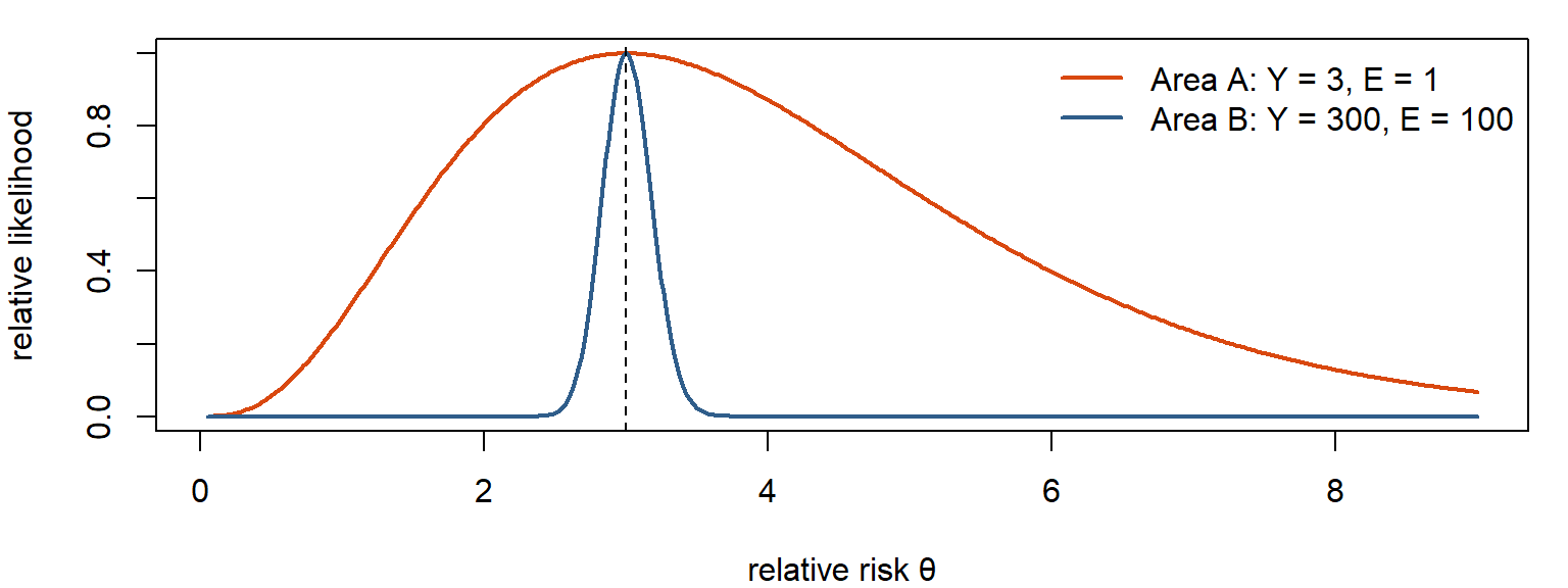
The key question on slide 3: when does a map reflect risk, and when does it reflect noise? Two areas with the same SMR of 3.0 can carry very different amounts of information (3 observed vs 1 expected, or 300 vs 100).

The answer is a Bayesian hierarchical model that lets areas borrow strength: from all areas (partial pooling, unstructured effects) and from their neighbours (spatial smoothing, structured effects). The BYM and BYM2 models combine the two. The output is not only a smoother map but a posterior distribution for every area’s relative risk, which gives credible intervals and exceedance probabilities.

NoteSources and session

Slides: “session_4_v0.pdf” (Qinyun Lin, 9 October 2026, 13:15–15:00).

Learning objectives (Canvas post): by the end of this session you should be able to

1. explain why crude small-area disease rates and standardized mortality ratios (SMRs) can be unstable;
2. recognize how the epidemiological outcome and denominator inform the choice of statistical likelihood;
3. explain the concepts of shrinkage, partial pooling and spatial smoothing;
4. describe the roles of spatially structured and unstructured random effects in BYM/BYM2 models;
5. interpret posterior relative risks, credible intervals and exceedance probabilities.

Key questions to think about (Canvas post), each answered in a section marked ❓:

1. Why might two geographic areas with the same SMR provide very different amounts of information about their underlying disease risks? → 4.1
2. What is the difference between partial pooling and spatial smoothing? → 4.9
3. Why does the BYM2 model include both spatially structured and unstructured variation? → 4.11
4. Why might an area with a higher estimated relative risk have weaker evidence of elevated risk than another area? → 4.17

Optional reading: Gómez-Rubio, Bayesian Inference with INLA, a free online book on latent Gaussian models, spatial models and their implementation in R. Not required; you are not expected to understand the computational details of INLA.

TipBefore you start: three ideas you need

Poisson regression with an offset. For counts Y with exposure (person-time) T: log E[Y] = log T + Xβ. The offset log T has coefficient fixed at 1, so the model describes the rate Y/T.

Bayes’ theorem in words. Posterior ∝ likelihood × prior: what you believe after the data combines what the data say with what you assumed before.

Random effects (from mixed models). Group-specific effects drawn from a common distribution, for example vᵢ ~ N(0, σ²). Groups with little data get estimates pulled toward the overall mean. Session 2’s Empirical Bayes smoothing is a simpler version of the same idea.

4.1 Same SMR, very different information

In short. An SMR of 3 based on 3 cases is mostly noise; based on 300 cases it is solid. The ratio hides how much data lies behind it.

Think of it as: Three heads in three coin flips says little about the coin; 300 heads in 400 flips says a lot.

	Area A	Area B
Observed Y	3	300
Expected E	1	100
SMR = Y/E	3.0	3.0
Uncertainty	Wide	Much narrower

Key question 1: why might two areas with the same SMR provide very different amounts of information? Because the information depends on the size of the counts, not the ratio. With Y ~ Poisson(Eθ), the standard error of the SMR is roughly √Y / E = SMR/√Y. Area A: 3/√3 ≈ 1.7; area B: 3/√300 ≈ 0.17, ten times smaller. One or two extra cases in A would change its SMR enormously; in B they hardly matter.

A sensible model should let the data-rich area speak more strongly than the data-poor one.

Likelihood for the relative risk θ (scaled to a maximum of 1) in two areas with the same SMR = 3. Area A (3 observed, 1 expected) is compatible with almost anything from 1 to 8; area B (300 observed, 100 expected) pins θ down near 3.

On the exam, be able to say: Same SMR, different information: the uncertainty depends on the size of the counts (SE ≈ SMR/√Y). Area A (3/1) is compatible with a wide range of risks; area B (300/100) is not.

4.2 Start with the estimand: which likelihood?

In short. Choose the model from the data: people with or without a condition out of N examined → Binomial; new events over time → Poisson with person-time; observed vs expected → Poisson with E.

First ask what is observed, what the denominator or reference is, and what quantity you want to estimate.

Outcome	Data	Likelihood	Target
Incidence / mortality	New events or deaths over population or person-time PTᵢ	Yᵢ ~ Poisson(PTᵢ λᵢ), i.e. log μᵢ = log PTᵢ + ηᵢ	Rate λᵢ
Prevalence	Existing cases among Nᵢ individuals examined	Yᵢ ~ Binomial(Nᵢ, pᵢ), logit(pᵢ) = ηᵢ	Probability pᵢ
Disease mapping with expected counts	Observed cases compared with an expected count Eᵢ	Yᵢ ~ Poisson(Eᵢ θᵢ)	Relative risk θᵢ

ηᵢ is the linear predictor on the log (or logit) scale: possibly covariates plus spatial effects.

For incidence, the offset log PTᵢ fixes the amount of exposure; the model estimates the rate.

Poisson or Binomial? Both outcomes are counts. The data structure decides the likelihood:

	Binomial	Poisson
Structure	Cases among a fixed number N of individuals, each yes/no	Events over exposure or person-time
Example (slide 8)	20 people with obesity out of 100 examined	15 deaths over 10,000 person-years
Target	Probability / prevalence pᵢ	Incidence or mortality rate λᵢ

A count of cases is not automatically Poisson. And BYM/BYM2 is a spatial random-effect structure, not intrinsically a Poisson model: it can be added to the linear predictor of either.

On the exam, be able to say: Incidence: Poisson(PTᵢλᵢ), target rate. Prevalence: Binomial(Nᵢ, pᵢ), target probability. Disease mapping: Poisson(Eᵢθᵢ), target relative risk. A count is not automatically Poisson; BYM2 can be used with either.

4.3 Observed and expected counts; indirect standardization

In short. The expected count is the number of cases the area would have if its people had the reference rates (by age and sex). Comparing observed with expected removes differences in age structure.

The classical disease-mapping model:

\[ Y_i \sim \text{Poisson}(E_i\,\theta_i) \]

In words: the observed count is random around expected count × relative risk; θᵢ is what we want to know.

Symbol	Meaning
Yᵢ	Observed number of cases or deaths in area i
Eᵢ	Expected cases if area i had the reference rates
θᵢ	Relative risk: θᵢ = 1 as expected; θᵢ > 1 elevated; θᵢ < 1 lower

The inferential target is the latent area-specific risk θᵢ.

Same model, two notations:

Disease-mapping notation	Regression notation
Yᵢ ~ Poisson(Eᵢ θᵢ), μᵢ = Eᵢ θᵢ	Yᵢ ~ Poisson(μᵢ), log μᵢ = log Eᵢ + ηᵢ, with ηᵢ = log θᵢ

log Eᵢ is the offset.

Where Eᵢ comes from: indirect standardization.

\[ E_i = \sum_a n_{ia}\, r^*_a \]

nᵢₐ is the population of area i in stratum a (for example age × sex) and r*ₐ the reference rate in that stratum. Eᵢ is the number of cases expected from the area’s own population composition. This lets you compare areas with different age structures: an area with many elderly residents is not flagged just for being old.

On the exam, be able to say: Eᵢ = Σₐ nᵢₐ r*ₐ (indirect standardization). Yᵢ ~ Poisson(Eᵢθᵢ) is a Poisson regression with offset log Eᵢ and log θᵢ as linear predictor.

4.4 The SMR as the crude estimate

In short. The SMR is the crude, unsmoothed estimate of the relative risk: simple, but unstable when E is small.

\[ \text{SMR}_i = Y_i / E_i \]

If each θᵢ is estimated separately, with no smoothing, the estimate is essentially the SMR (the maximum likelihood estimate of θᵢ under the Poisson model).

Strength	Problem
Simple, transparent, easy to map	Small denominators can produce extreme, unstable estimates

Extreme ≠ necessarily high underlying risk. An area with E = 0.5 and Y = 2 has SMR = 4, and with Y = 0 has SMR = 0, both from essentially no information. The variance of the SMR is roughly θᵢ/Eᵢ: the smaller Eᵢ, the noisier.

On the exam, be able to say: SMRᵢ = Yᵢ/Eᵢ, the estimate of θᵢ without smoothing. Simple and transparent, but extreme values from small denominators need not mean high risk.

4.5 One Bayesian idea: combine data with a model for plausible risks

In short. Bayesian disease mapping combines what each area’s data say with a model of how areas relate, giving an updated estimate with uncertainty.

\[ \text{posterior} \;\propto\; \text{likelihood} \times \text{prior} \]

Part	Role in disease mapping
Likelihood	What the observed counts say about each area’s risk
Prior / latent model	How areas are allowed to share information about their underlying risks
Posterior	Updated uncertainty about each area’s underlying risk

The key modelling decision: how should information be shared across areas? Not at all (SMR), with all areas equally (unstructured), or more with neighbours (spatial).

On the exam, be able to say: Posterior ∝ likelihood × prior. The key modelling decision is how areas share information.

4.6 Partial pooling and shrinkage

In short. Partial pooling: each area’s estimate is a compromise between its own data and the common pattern. Little data → pulled more (shrinkage).

Think of it as: Restaurant ratings again: few reviews → trust the typical rating more; many reviews → trust the restaurant’s own rating.

Extreme, noisy estimates move toward the common pattern.

Area	Crude	Smoothed	Why
A	3.00	1.45	Little information → strong shrinkage
B	3.00	2.75	Much information → little shrinkage
C	0.25	0.75	Little information → pulled up toward the mean

Illustrative numbers from slide 15.

Figure 1: Shrinkage with the illustrative numbers from slide 15. Areas A and B have the same crude SMR of 3.0, but A has little data and is pulled far toward the overall level, while data-rich B keeps most of its signal. Area C’s very low crude value is pulled up.

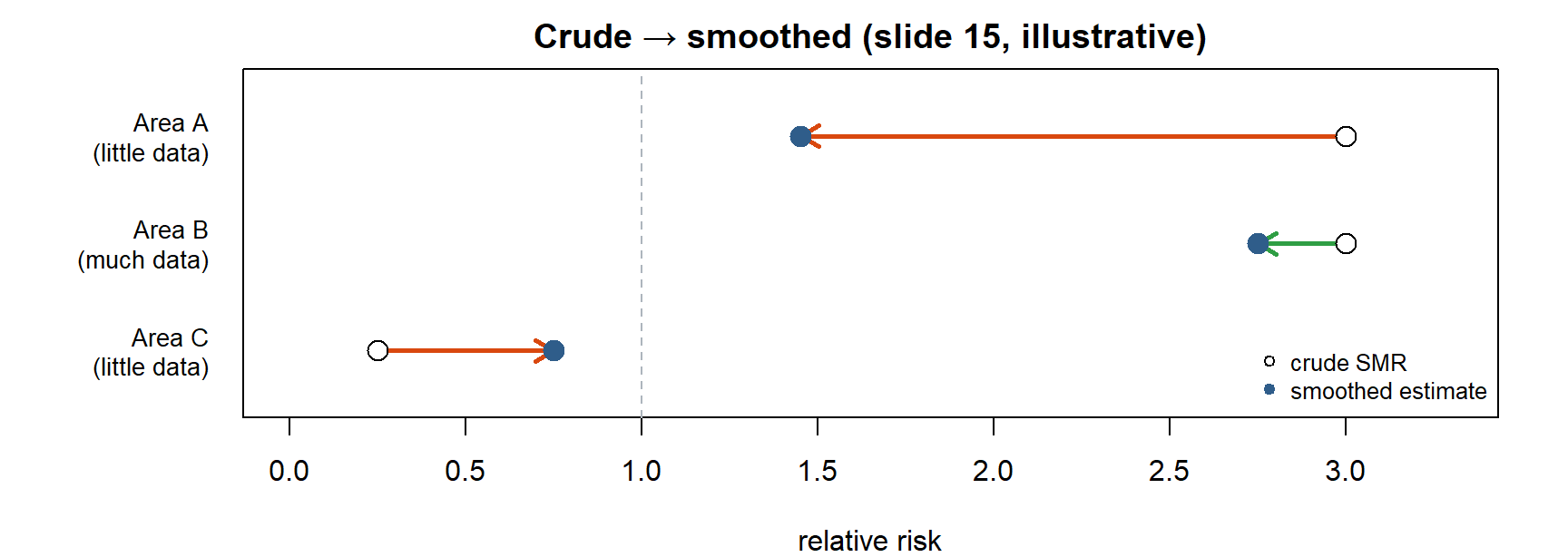
• Less information → more shrinkage.
• More information → less shrinkage.

Shrinkage is not “making areas equal.” It weights noisy area-specific information against a shared model. A data-rich area with a real excess keeps it.

The three ways of pooling:

	No pooling	Partial pooling	Complete pooling
Estimate	Each area alone (SMR)	Compromise, weighted by information	One common rate for all
Problem	Noisy	(the goal)	Ignores real differences

Try it. Simulate 50 areas with true relative risks around 1, very different expected counts, and compare crude SMRs with a simple partial-pooling estimate (a Poisson–gamma Empirical Bayes estimate, the closed-form cousin of the Bayesian models below).

The smoothed estimates for small-E areas collapse toward the overall level; large-E areas barely move. Plots side by side make the comparison direct.

On the exam, be able to say: Shrinkage moves noisy estimates toward the common pattern: data-poor areas shrink more, data-rich areas keep their signal. It is weighting, not making areas equal.

4.7 Unstructured heterogeneity: areas differ independently

In short. An unstructured random effect lets each area differ from the average, regardless of where it lies. It shrinks toward the overall mean but ignores geography.

\[ \log \theta_i = \alpha + v_i, \qquad v_i \sim \text{Normal}(0, \sigma_v^2) \]

In words: each area’s log relative risk = a common level + its own deviation, and all deviations come from one shared bell curve.

What vᵢ captures	Area-specific deviations from the overall level of risk α
What it does not use	No neighbourhood information: vᵢ and vⱼ are independent a priori
Result	A shared distribution → partial pooling: shrinkage, but not spatial smoothing

Every area is shrunk toward the same global level, regardless of where it is. This is the fully Bayesian version of Session 2’s Empirical Bayes idea.

On the exam, be able to say: log θᵢ = α + vᵢ, vᵢ ~ N(0, σᵥ²), independent: partial pooling (shrinkage) but no spatial smoothing.

4.8 Spatial smoothing: the CAR / ICAR prior

In short. The spatial (ICAR) prior says: an area’s hidden risk is probably close to the average of its neighbours’. Areas with many neighbours borrow more.

Think of it as: Guessing a house’s price from the houses on the same street.

Geography matters: neighbouring areas may share latent risk because they share

• environment (air pollution, built environment, climate);
• social context (deprivation, housing, local norms);
• healthcare (access, catchments, diagnostic practice);
• unmeasured factors (spatially patterned determinants not in X).

A spatial prior lets neighbouring areas share information about their underlying risks. In the conditional autoregressive form, an area’s latent effect is centred on its neighbours:

\[ u_i \mid u_{-i} \;\sim\; \text{Normal}\!\left(\frac{\sum_j w_{ij} u_j}{n_i},\; \frac{\sigma_u^2}{n_i}\right) \]

In words: given its neighbours, an area’s spatial effect is expected to be near their average, and the more neighbours it has, the closer.

Part	Meaning
Neighbour mean Σⱼwᵢⱼuⱼ / nᵢ	The conditional centre is set by adjacent areas
nᵢ	Number (or total weight) of neighbours
Conditional variance σᵤ²/nᵢ	More neighbours → greater conditional precision (under the standard intrinsic CAR, ICAR, specification)

Intuition (slide 18). If A and C have similar spatial effects, the prior encourages B, between them, to be similar, unless B’s own data strongly disagree. This is borrowing strength through geography.

For this course: understand the mechanism; you do not need to derive the joint distribution.

On the exam, be able to say: ICAR: uᵢ given the others is normal with mean = average of the neighbours’ u and variance σᵤ²/nᵢ. More neighbours, more conditional precision. Borrowing strength through geography.

4.9 Partial pooling vs spatial smoothing

In short. Partial pooling borrows from all areas; spatial smoothing borrows from neighbours.

Key question 2: what is the difference between partial pooling and spatial smoothing?

	Partial pooling (unstructured vᵢ)	Spatial smoothing (structured uᵢ)
Shrink toward	The global mean of all areas	The local mean of each area’s neighbours
Uses the map?	No: shuffling the areas on the map changes nothing	Yes: the neighbourhood graph W decides who borrows from whom
Captures	Area-specific, non-spatial heterogeneity	Smooth, clustered geographic patterns
Model	Hierarchical model with exchangeable effects	CAR / ICAR prior

Figure 2: Simulated map of 100 small areas (expected counts 0.5 to 15). The raw SMR map is speckled with noise. Unstructured pooling shrinks every area toward the global mean, so noise is reduced but the map ignores geography. Spatial smoothing pulls each area toward its neighbours and recovers the true pattern best. Illustrative Poisson–gamma estimates, not a fitted BYM2 model.

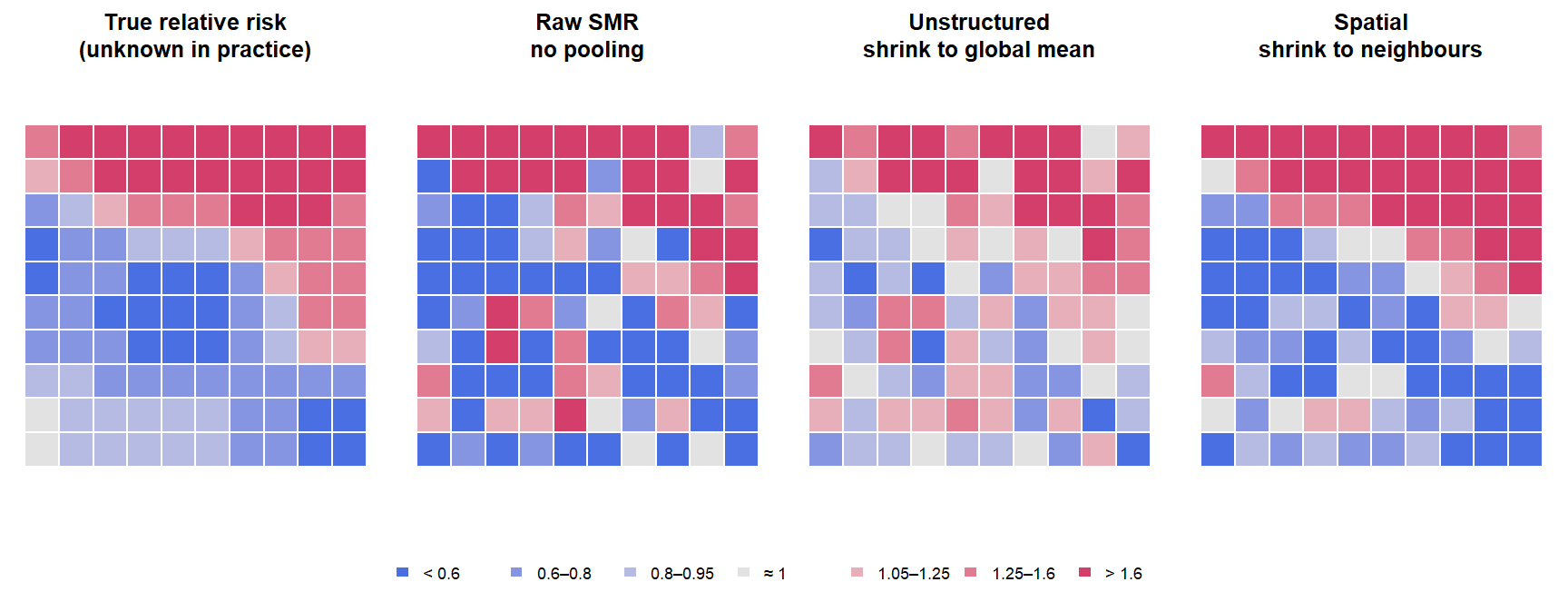
Both shrink noisy small-area estimates. Spatial smoothing is a particular kind of partial pooling where the “group” an area borrows from is its neighbourhood.

On the exam, be able to say: Unstructured pooling shrinks toward the global mean and ignores the map; spatial smoothing shrinks toward the neighbourhood mean using W. Spatial smoothing is a geographic form of partial pooling.

4.10 The neighbourhood graph returns, in a different role

In short. The same neighbour list W returns, but now it says which areas’ hidden risks should be similar, not how observed values are linked.

Earlier: Moran’s I, SAR, SEM	Here: Bayesian disease mapping
W summarises observed neighbouring values, or links outcomes / errors through a spatial process	Adjacency defines which latent area effects are encouraged to be similar
Spatial lag or error structure	A spatial prior for latent effects

Same neighbourhood graph, different role in the statistical model.

4.11 The Besag–York–Mollié (BYM) model: why both uᵢ and vᵢ

In short. BYM = overall level + a spatial part (neighbours similar) + a non-spatial part (area-specific deviations).

Think of it as: Your height = what you share with your family + what is just you. Leave out either part and the explanation is wrong.

\[ Y_i \sim \text{Poisson}(E_i \theta_i), \qquad \log \theta_i = \alpha + u_i + v_i \]

In words: log relative risk = common level + a part shared with neighbours + a part that is the area’s own.

Term	Role
α, overall level	Baseline log relative risk
uᵢ, structured	Spatially correlated component (ICAR): neighbouring areas borrow strength
vᵢ, unstructured	Independent area-specific heterogeneity

Two kinds of residual variation: spatial pattern + local noise. The model is named after Besag, York & Mollié (1991) (original paper, not required). Not all between-area variation needs to be spatially structured.

Key question 3: why include both structured and unstructured variation?

• Structured uᵢ captures smooth or clustered geographic pattern: if one area is high, its neighbours are compatible with being high.
• Unstructured vᵢ captures area-specific departures that do not need to resemble neighbours: local heterogeneity remains possible.
• Without vᵢ, every residual difference is pushed into the spatial surface: a genuinely odd area would be forced to look like its neighbours (over-smoothing), and its neighbours distorted toward it.
• Without uᵢ, geography is ignored: only global shrinkage.

Including both lets the data decide how much of the extra variation is spatial.

Both components represent unexplained variation in underlying risk; the distinction between them is statistical, not a claim about causes.

On the exam, be able to say: log θᵢ = α + uᵢ + vᵢ: uᵢ structured (ICAR), vᵢ unstructured. Without vᵢ everything is forced into the spatial surface (over-smoothing); without uᵢ geography is ignored.

4.12 BYM2: separating overall variability from the spatial fraction

In short. BYM2 rewrites BYM with two easy dials: τ, how much unexplained variation there is overall, and ρ, how much of it is spatial (0 = none, 1 = all).

Think of it as: A volume knob (τ: how much variation) and a balance knob (ρ: spatial vs non-spatial).

The problem with classic BYM (slide 23):

• the marginal variability of uᵢ depends on the entire neighbourhood graph;
• unlike vᵢ, its variance parameter does not directly represent marginal variability;
• so how much residual variation is spatially structured is not directly interpretable, and priors are hard to set.

BYM2 reparameterizes the same idea:

\[ \log \theta_i = \alpha + \frac{1}{\sqrt{\tau}}\left(\sqrt{\rho}\; u_i^{*} + \sqrt{1 - \rho}\; v_i\right) \]

In words: the same two parts as BYM, but mixed with a balance dial ρ (how much is spatial) and scaled by one volume dial 1/√τ (how much unexplained variation in total).

Parameter	Meaning
τ, overall precision	1/√τ controls the overall magnitude of residual heterogeneity. Larger τ → less residual variability; smaller τ → more
ρ, spatial fraction (mixing parameter), 0 ≤ ρ ≤ 1	ρ close to 1 → mostly structured; ρ close to 0 → mostly unstructured
uᵢ*, scaled spatial effect	Scaled so its variance has a stable interpretation across graphs (marginal variance about 1, like vᵢ)

This is the parameterization commonly used in modern Bayesian disease mapping. Original paper (not required): Riebler et al. (2016).

Interpreting ρ:

ρ ≈ 0	ρ ≈ 0.5	ρ ≈ 1
Residual heterogeneity is predominantly unstructured	Both components matter	Residual heterogeneity is dominated by geographic structure

Figure 3: What the BYM2 mixing parameter ρ does, simulated on a 12 × 12 grid. The same structured component u* (an ICAR draw) and unstructured component v, mixed as √ρ·u* + √(1−ρ)·v. With ρ = 0 the residual pattern is pure speckle; with ρ = 1 it is a smooth surface where neighbours resemble each other.

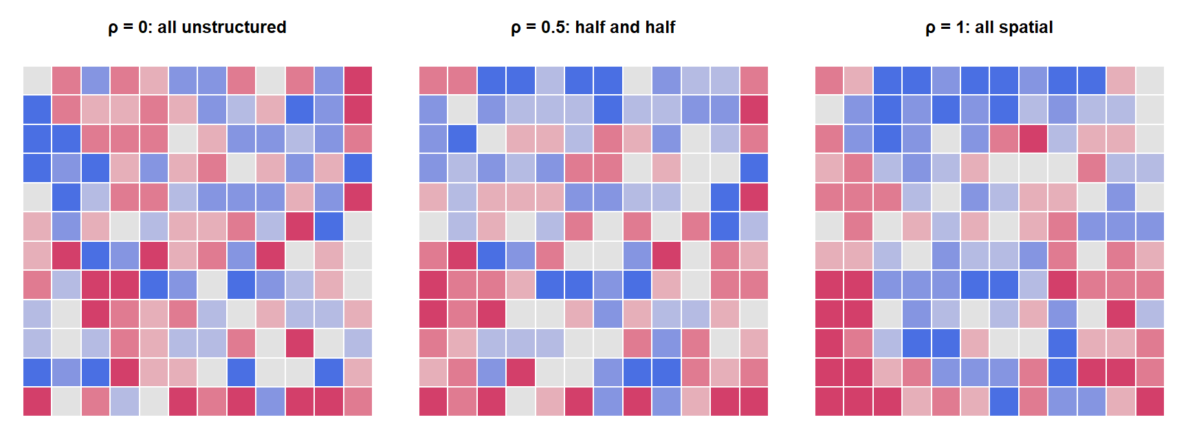
The slide’s question: if ρ is estimated as 0.9, does it mean 90% of disease cases are caused by spatial factors? No. ρ describes the residual latent variation (what remains after α and any covariates) on the BYM2 mixing scale: about 90% of the unexplained between-area variance is spatially structured. It says nothing about causes, nothing about cases, and nothing about variation that the covariates already explain. Also, BYM2’s ρ is not SAR’s ρ (3.4).

Little residual variation overall, and most of it is spatially structured

Much residual variation overall, and most of it is unstructured noise

About 85% of all cases in the region are caused by spatial factors

The covariates explain 85% of the variation between the areas

τ is a precision, so a large τ means small residual variability. ρ near 1 means the residual variation that exists is mostly structured. ρ is not a causal share of cases and not an R².

On the exam, be able to say: BYM2: log θᵢ = α + (1/√τ)(√ρ·uᵢ* + √(1−ρ)·vᵢ). Larger τ = less residual variation. ρ is the share of residual variation that is spatially structured, not the share of disease caused by space.

4.13 Priors: what are we putting priors on?

In short. Priors go on the fixed effects, the overall variability and the spatial share. They decide how much and what kind of smoothing happens.

Part	Prior
Fixed effects α, β	Usually weakly informative or context-appropriate
Overall variability	Prior on τ (or the residual standard deviation 1/√τ)
Spatial mixing	Prior on ρ: expresses assumptions about the balance between structured and unstructured variation

For an introductory course, the key point is that priors regularize complexity. In applied work, consider prior sensitivity.

• A prior on the overall variability influences how much smoothing occurs.
• A prior on the spatial mixing influences the type of smoothing.

On the exam, be able to say: A prior on the overall variability affects how much smoothing occurs; a prior on the mixing parameter affects the type of smoothing. Priors regularize complexity; check sensitivity.

4.14 Penalized-complexity (PC) priors

In short. PC priors prefer the simpler model unless the data clearly ask for more.

Marked optional depth on the slide.

Idea: start from a simpler base model (for BYM2: no residual variation, or no spatial structure) and penalise departures from it, so complexity is only used when the data support it. Original paper (not required): Simpson et al. (2017).

Why useful: hyperpriors can be stated as interpretable probability statements about plausible effect sizes, for example “P(residual SD > 1) = 0.01” or “P(ρ < 0.5) = 2/3”, rather than arbitrary values for a precision parameter. This is a common strategy with INLA and BYM2.

4.15 Adding area-level covariates

In short. Covariates can be added; exp(β) is the ratio of relative risks per unit of x. It is still an area-level, not causal, association.

\[ \log \theta_i = \alpha + X_i\beta + u_i + v_i \]

In words: as BYM, plus a covariate; exp(β) is how many times higher the relative risk is per unit of x.

β	Area-level association with relative risk, on the log scale
exp(β)	Relative-risk ratio for a one-unit difference in X, conditional on the model
Caution	Spatial random effects do not automatically solve confounding or make β causal

Disease mapping and ecological regression overlap, but the inferential question matters: estimating each area’s risk (mapping) or estimating an area-level association (regression).

Spatial confounding. If X itself is spatially smooth, X and the spatial effect uᵢ can explain the same geographic pattern; adding uᵢ can then change β a lot, and neither version is automatically “right”.

On the exam, be able to say: exp(β) = relative-risk ratio for a one-unit difference in X, conditional on the model. Spatial random effects do not remove confounding or make β causal.

4.16 What the posterior gives: relative risks, credible intervals, exceedance

In short. For every area the model gives a whole distribution of possible risks. Summarise it as a point estimate, a credible interval and the probability that risk exceeds a threshold.

Output	What it is	Answers
Posterior mean / median of θᵢ	A smoothed point estimate; often mapped as relative risk	How high is the risk?
Credible interval (CrI)	Range of posterior uncertainty for θᵢ	How sure are we?
Exceedance probability P(θᵢ > c ∣ data)	Probability that θᵢ exceeds a scientifically meaningful threshold c	How likely is it that risk is elevated?

Bayesian disease mapping lets you map uncertainty, not only point estimates.

Interpreting a 95% credible interval. Example: posterior 95% CrI for θᵢ = [1.08, 1.42]. Under the fitted model and priors, 95% of the posterior probability for this area’s (latent) relative risk lies between 1.08 and 1.42.

A credible interval is	It is not
A probability statement about the parameter, given the data, model and prior	“95% of repeated confidence intervals contain the fixed true value” (the frequentist confidence interval statement)
Conditional on the model, data and prior assumptions	A statement free of assumptions

Exceedance probabilities.

Threshold	Meaning
c = 1	Probability that risk is above the reference level
c = 1.2	Probability that risk exceeds a 20% elevation

The choice of c should be tied to the scientific or decision context, not chosen to make a map look interesting. A map of exceedance probabilities can be more informative than thresholding a map of point estimates. A common convention flags areas with P(θᵢ > 1) above 0.8 or 0.95.

On the exam, be able to say: Posterior mean/median (smoothed RR), 95% credible interval (95% posterior probability given model and priors; not the confidence-interval statement), exceedance probability P(θᵢ > c | data).

4.17 Higher posterior RR does not always mean stronger evidence

In short. A bigger estimate is not stronger evidence. Look at the interval and the exceedance probability too.

	Area A	Area B
Posterior mean RR	1.30	1.20
95% CrI	0.75–2.00	1.10–1.31
P(RR > 1)	0.72	0.995

Figure 4: Posterior distributions for the two areas on slide 32, approximated by log-normal curves matching the slide’s 95% credible intervals. Area A’s distribution is wide, so a large share lies below 1. Area B’s is narrow and almost entirely above 1. The shaded area is the exceedance probability P(θ > 1); with this approximation A’s is 0.79 rather than the slide’s 0.72.

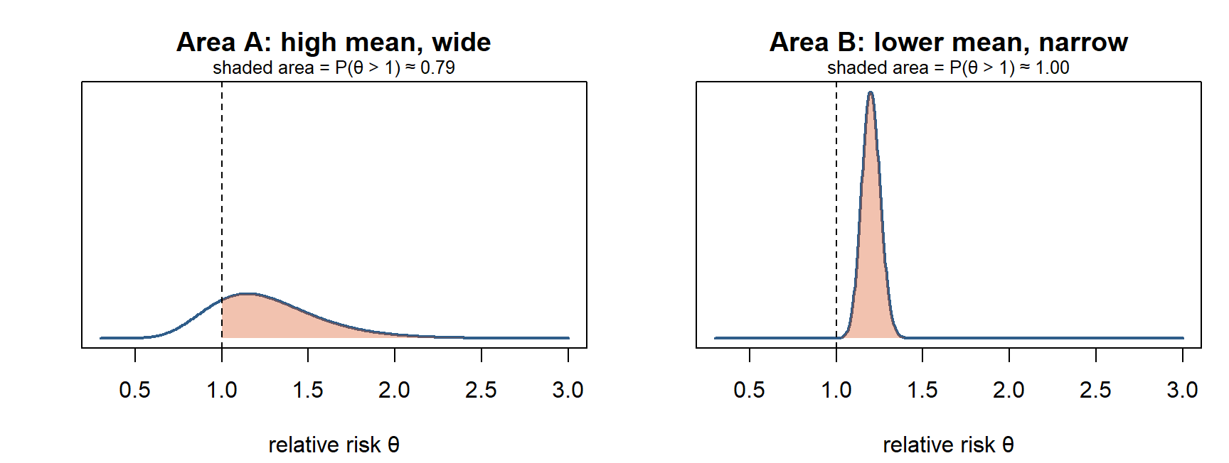
Which area gives stronger evidence of elevated risk? Area B. A has the higher point estimate, but its interval includes 1 and P(RR > 1) is only 0.72. B’s estimate is lower but precise, entirely above 1.

Key question 4: why might an area with a higher estimated RR have weaker evidence of elevated risk? Because magnitude and certainty are different dimensions. A small area (few expected cases) has a wide posterior: even after shrinkage its mean can be high while the data are compatible with no excess. A large area can have a modest but precisely estimated excess.

On the exam, be able to say: Magnitude and certainty are different: a small area can have a high posterior mean with a wide interval (weak evidence), a large area a modest but precise excess (strong evidence).

4.18 Raw SMR → non-spatial smoothing → spatial smoothing

In short. Raw SMR: no borrowing. Unstructured model: borrow from all areas. BYM/BYM2: borrow from all areas and from neighbours.

	Raw SMR	Unstructured model	BYM / BYM2
Each area	Stands alone	Partially pools toward an overall distribution	Partial pooling + neighbouring areas inform the structured component
Sparse counts	Very sensitive	Stabilised	Stabilised
Uses geography	No	No	Yes, explicitly
Uncertainty	Only frequentist CI per area	Posterior for each area	Posterior for each area

The gain is not merely a prettier map: it is a model-based estimate of latent risk with uncertainty. Unstructured hierarchical models borrow through a shared distribution; BYM2 additionally uses spatial relationships.

On the exam, be able to say: The gain is a model-based estimate of latent risk with uncertainty, not just a prettier map.

4.19 Cautions: smoothing can hide real boundaries; islands

In short. Smoothing assumes neighbours are alike. Where a real border separates them, or an area has no neighbours, it can mislead.

Spatial smoothing can hide real boundaries (slide 34):

• administrative neighbours need not share the same underlying process;
• a river, road, policy boundary or healthcare catchment may create a real discontinuity;
• strong smoothing can attenuate sharp local signals (a single polluted area, a point source);
• so the adjacency definition is a substantive modelling choice.

Borrowing strength helps when the borrowing assumption is plausible.

Islands / areas with no neighbours (slide 35). An ICAR component is defined through the neighbourhood graph, so an isolated area has no adjacency information to borrow from. Handling: check the graph carefully; define meaningful connections when scientifically justified (for example a ferry link); otherwise rely on the unstructured component or the software’s handling. Always inspect the neighbourhood graph before fitting. (Compare isolates in Session 2.)

On the exam, be able to say: Smoothing can hide real discontinuities (rivers, catchment borders) and attenuate sharp local signals; the adjacency definition is a substantive choice. Islands have no neighbours to borrow from.

4.20 Workflow and model checking

In short. Define the outcome, build the neighbour graph, fit, check, and report risk with its uncertainty.

flowchart LR
  A["1 · Define outcome<br/>incidence? prevalence?<br/>observed/expected?"] --> B["2 · Build graph<br/>meaningful<br/>neighbourhood structure"]
  B --> C["3 · Fit model<br/>Poisson/Binomial + BYM2;<br/>consider covariates"]
  C --> D["4 · Check<br/>sensitivity, fit, residual<br/>pattern, prior influence"]
  D --> E["5 · Communicate<br/>map risk AND uncertainty;<br/>interpret cautiously"]

Workflow: each arrow means “then”. Not causal. A practical Bayesian disease-mapping analysis (slide 37).

What to check after fitting (slide 38):

Check	Question
Posterior predictive fit	Can the fitted model reproduce relevant features of the observed data?
Residual structure	Is meaningful spatial pattern still unexplained?
Sensitivity	Do conclusions change with priors, graph choices or model specification?
Complexity	Do extra components improve inference enough to justify them?

Posterior maps are the beginning of interpretation, not the end of model checking. A model is one part of the epidemiological argument, not the entire argument.

4.21 Why INLA is common

In short. INLA is a fast way to compute the results of models like BYM2. The details are not part of the course.

You are not expected to understand the computational details of INLA (Canvas post).

Latent Gaussian models	BYM/BYM2 fit naturally in this framework
Fast approximation	INLA (integrated nested Laplace approximation) approximates posterior marginals without running conventional MCMC
Practical workflow	R-INLA supports adjacency graphs, BYM2, priors, posterior summaries and predictions

INLA is a computational approach: it does not change the model, only how the posterior is approximated. Original paper (not required): Rue, Martino & Chopin (2009).

Optional reading (Canvas post): Gómez-Rubio, Bayesian Inference with INLA. Not required reading.

4.22 A high-risk area is not a causal explanation

In short. A high-risk area on a map is a description, not a cause.

Caution	Why
Ecological inference	Area-level associations need not represent individual-level relationships (ecological fallacy, 1.11)
Spatial confounding	Covariates and latent spatial effects can share similar geographic patterns
MAUP / boundaries	Results depend on how areas are defined and aggregated (1.10)

“This area has elevated posterior risk” ≠ “living here causes the disease.”

Spatial regression vs disease mapping ask related but different questions:

Spatial regression (Session 3)	Bayesian disease mapping (Session 4)
How should regression change when observations are spatially dependent?	How can we estimate underlying area risk when counts are noisy and geographically structured?
Focus: association, dependence, residual structure	Focus: latent risk, smoothing, uncertainty

Both require you to make the spatial mechanism explicit.

On the exam, be able to say: Elevated posterior risk ≠ causal explanation: ecological inference, spatial confounding and the MAUP all limit interpretation.

4.23 Checkpoint: reconstruct the logic

Slide 41 asks you to explain each arrow in one sentence. Try it before opening the answer.

flowchart LR
  A["Observed /<br/>expected"] --> B["SMR"] --> C["Poisson<br/>model"] --> D["Partial<br/>pooling"] --> E["CAR /<br/>ICAR"] --> F["BYM2"] --> G["Posterior risk<br/>+ uncertainty"]

Lecture map: each arrow is one step of the argument. Not causal.

NoteModel answer: one sentence per arrow

1. Observed/expected → SMR: dividing observed by expected cases (from indirect standardization) gives a crude relative risk that adjusts for population composition.
2. SMR → Poisson model: treating Yᵢ ~ Poisson(Eᵢθᵢ) makes the SMR the maximum likelihood estimate of θᵢ and shows that its uncertainty depends on the size of the counts.
3. Poisson model → partial pooling: giving the log relative risks a common distribution lets data-poor areas borrow from the others, shrinking unstable SMRs toward the overall level.
4. Partial pooling → CAR/ICAR: a spatial prior centres each area’s effect on its neighbours’ effects, so borrowing happens locally (spatial smoothing).
5. CAR/ICAR → BYM2: combining a scaled structured effect with an unstructured effect, mixed by ρ and scaled by τ, lets the data decide how much residual variation is spatial.
6. BYM2 → posterior risk + uncertainty: the fitted model gives a posterior for each θᵢ, summarised as posterior means, credible intervals and exceedance probabilities.

4.24 Take-home messages and key questions

1. Start with the estimand. Incidence, prevalence and standardized burden imply different data structures.
2. Raw small-area rates are noisy. SMRs can be extreme simply because denominators are small.
3. Bayesian models partially pool. Data-poor areas shrink more; data-rich areas keep more of their own signal.
4. BYM2 separates two ideas: overall heterogeneity and the fraction that is spatially structured.
5. Map uncertainty too. Posterior RR, credible intervals and exceedance probabilities answer different questions.

NoteWhy is Empirical Bayes (Session 2) not the same as BYM2?

EB estimates the prior from the data and shrinks every area toward one global rate, giving point estimates only. BYM2 is fully Bayesian: it puts priors on the hyperparameters, gives a full posterior for every area, and includes a spatial component, so areas are also smoothed toward their neighbours.

NoteWhen could spatial smoothing give a misleading map?

When neighbouring areas do not share the same underlying process: a real boundary (river, motorway, catchment border, policy line) or a sharp local hazard. The ICAR prior pulls the high area down and its neighbours up, blurring a genuine signal. Check the adjacency definition and compare with a less smoothed model.

NotePrevalence of diabetes from a health survey in each region: Poisson or Binomial?

Binomial: Yᵢ people with diabetes out of Nᵢ respondents, each yes/no, with target pᵢ (logit link). A BYM2 term can still be added to logit(pᵢ). Poisson would fit new diagnoses over person-time.