Session 3 — Introduction to Spatial Regression

OLS with spatial data · residual autocorrelation · the spatial lag Wy · spatial lag model (SAR) and its impacts · spatial error model (SEM) · diagnostics and model choice

Session 2 asked whether nearby values resemble one another. Session 3 asks the regression question: how should a regression model change when observations are spatially dependent?

The starting point is ordinary least squares (OLS). If, after adjusting for covariates, the residuals of neighbouring areas still resemble each other, the model has left something spatial unexplained. There are two classic ways to put spatial dependence into the model, and they tell different scientific stories:

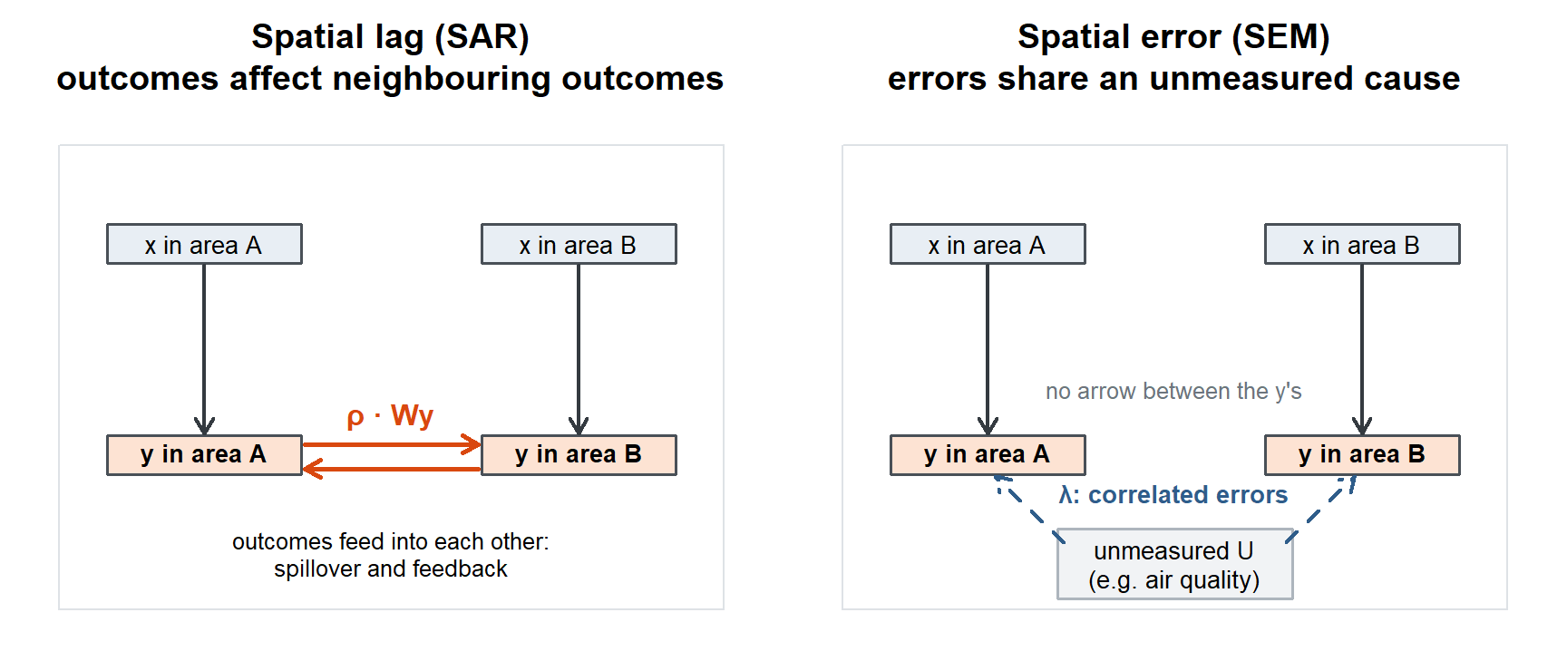
the spatial lag model (SAR): an area’s outcome depends on its neighbours’ outcomes (interaction, diffusion, feedback);
the spatial error model (SEM): the errors are spatially correlated (unmeasured, spatially patterned determinants).

The session’s emphasis is conceptual: what ρ and λ mean, why SAR coefficients cannot be read like OLS coefficients, and how to reason about model choice. No estimator derivations.

Sources and session

Slides: “session_3_v0-1.pdf” (Qinyun Lin, 9 October 2026, 10:15–12:00).

Learning goals (slide 4): by the end of the session you should be able to

recognize why spatial dependence can matter in regression;
distinguish spatial lag (SAR) from spatial error (SEM) conceptually;
interpret what ρ and λ represent, without deriving estimators;
diagnose residual spatial autocorrelation and think about model choice.

Optional viewing: Luc Anselin, Applied Spatial Regression Analysis (YouTube playlist, 13 lectures). A step-by-step introduction to spatial regression; it also covers more advanced topics than STA530. The lectures that match a section are linked in a Watch box at the end of that section; the full list is on Resources.

Before you start: three ideas you need

Residuals. eᵢ = yᵢ − ŷᵢ, the part of the outcome the covariates did not explain. OLS assumes the errors are independent of each other.

The spatial lag from Session 2. With a row-standardized weights matrix W, (Wy)ᵢ = Σⱼ wᵢⱼ yⱼ is the average of area i’s neighbours. See 2.8.

Geometric series. 1 + ρ + ρ² + ρ³ + … = 1/(1 − ρ) when |ρ| < 1. The matrix version explains SAR feedback.

3.1 OLS with spatial data: the assumption that can fail

In short. Ordinary regression assumes that what the model misses (the residuals) is unrelated between observations. With areas, neighbouring residuals are often alike, which makes standard errors too small and can bias the results.

The familiar model:

\[ y = X\beta + \varepsilon . \]

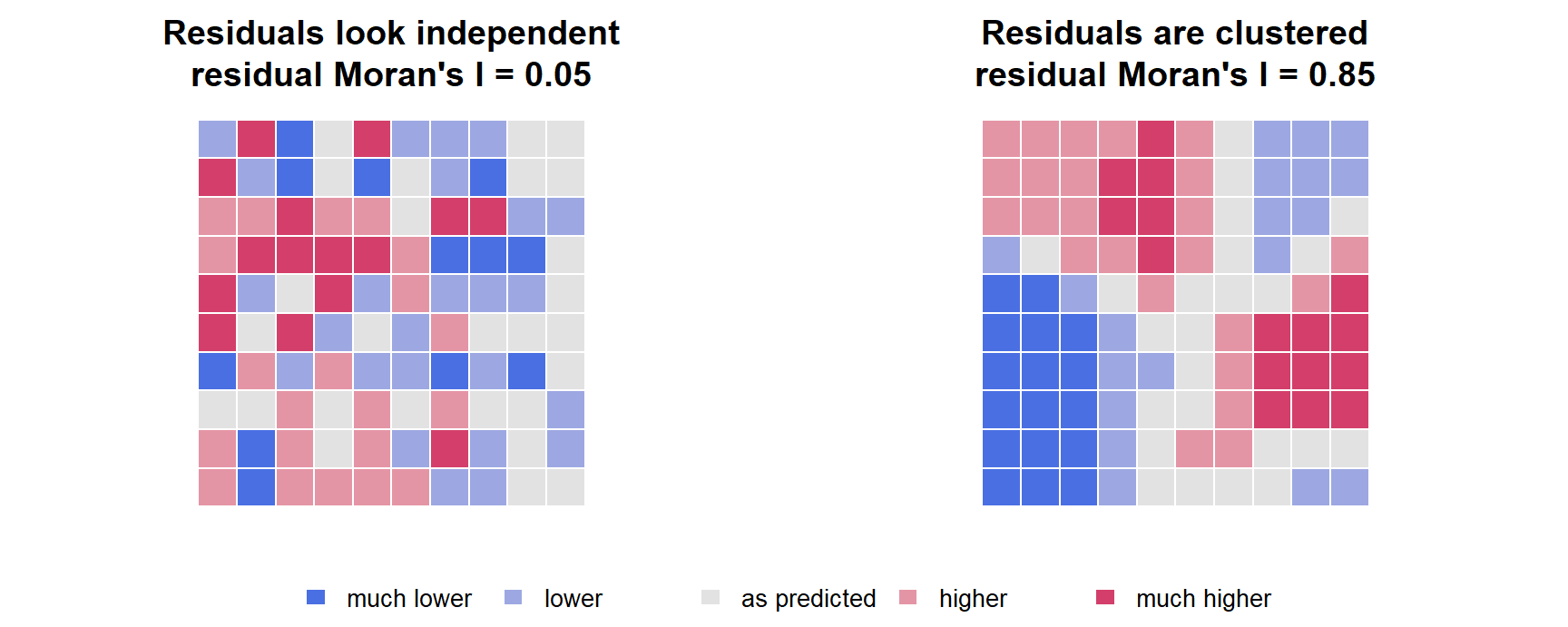
Key assumption here: after accounting for X, there is no remaining spatial dependence in the errors. Spatial data give a reason to doubt that: the slide shows the same regression equation with two very different residual maps, one that looks random and one with clear clusters of positive and negative residuals.

Figure 1: Two residual maps from the same kind of regression, simulated. Left: residuals scattered at random, residual Moran’s I near 0, the OLS assumption looks fine. Right: positive residuals cluster in some regions and negative in others, residual Moran’s I is high, so something spatial was left out of the model.

Why it matters:

Standard errors. With positively autocorrelated residuals, neighbouring areas carry overlapping information. OLS treats them as independent, so it typically understates the uncertainty: standard errors too small, p-values too small.
Bias. If the spatial pattern comes from a spatial process in the outcome (SAR) or from an omitted spatially patterned confounder, the coefficients themselves can be biased.
Science. Clustered residuals say the model has missed something that is organised in space.

“If I include enough covariates, spatial dependence goes away.” Sometimes, if the covariates capture the spatial process. But clustered residuals can remain after adjustment, and the next step is to ask why (3.2), not to add variables blindly.

On the exam, be able to say: OLS assumes no remaining spatial dependence in the errors after accounting for X. Spatially autocorrelated residuals mean understated uncertainty and possibly biased coefficients.

3.2 After adjustment, neighbouring residuals are similar: what could it mean?

In short. If residuals still cluster after adjustment, ask why: outcomes spreading between areas, a missing spatially patterned factor, or a wrongly specified model.

The slide’s example: area-level cardiovascular mortality modelled with age structure, income, smoking prevalence and urbanicity. After adjustment, neighbouring areas still have similar residuals. Possible explanations:

	Explanation	Model it points to
A	A spatial process links outcomes across areas (one area’s outcome affects its neighbours’)	Spatial lag (SAR)
B	An omitted determinant is spatially patterned (pollution, access to care, deprivation not fully measured)	Spatial error (SEM)
C	Something else: misspecification (wrong functional form, a missing nonlinear term), spatial heterogeneity (the relationship differs across regions), wrong scale	Fix the model; heterogeneity models (outside the course)

For cardiovascular mortality, A is hard to defend (deaths in one area do not cause deaths next door). B and C are more plausible.

On the exam, be able to say: Three explanations: a spatial process linking outcomes (SAR), an omitted spatially patterned determinant (SEM), or misspecification/heterogeneity.

3.3 The new ingredient: the spatially lagged outcome Wy

In short. Wy is simply “the average outcome of my neighbours”.

W defines who is a neighbour and how much each counts (Session 2).
y is the outcome in every area.
Wy is the spatially lagged outcome: for each area, a weighted summary of its neighbours’ y.

If W is row-standardized, (Wy)ᵢ is roughly the average outcome among area i’s neighbours.

Four areas in a row A – B – C – D, rook neighbours, row-standardized:

Area	Neighbours	wᵢⱼ	y	(Wy)ᵢ
A	B	1	10	14
B	A, C	½, ½	14	(10 + 18)/2 = 14
C	B, D	½, ½	18	(14 + 30)/2 = 22
D	C	1	30	18

3.4 The spatial lag model (SAR) and ρ

In short. SAR adds the neighbours’ average outcome as a predictor: y depends on the y next door. ρ says how strongly.

Think of it as: Contagion: an area’s rate rises when its neighbours’ rates rise.

\[ y = \rho W y + X\beta + \varepsilon \]

In words: an area’s outcome = ρ times its neighbours’ average outcome + the usual covariate part + noise.

Parameter	Meaning
ρ (rho), spatial dependence	How strongly outcomes are linked through W. ρ = 0 gives back OLS; ρ > 0 means an area’s outcome rises with its neighbours’ outcomes
β, covariates	Association with X, conditional on the spatial process
ε, remaining noise	Assumed independent

Key idea: y in one area is jointly determined with y in neighbouring areas. y appears on both sides: that is why OLS cannot simply be applied with Wy as an extra covariate (Wy is correlated with ε; the model is estimated by maximum likelihood or other methods outside the course).

Mechanisms that make SAR plausible: interaction, diffusion, feedback, where the outcome itself spreads.

Watch: Luc Anselin’s lecture on this

▶ Spatial Regression Specifications: the lag and error models side by side

Optional, from the Canvas post. Luc Anselin’s lecture series Applied Spatial Regression Analysis goes beyond STA530 in places.

On the exam, be able to say: SAR: y = ρWy + Xβ + ε. ρ measures how strongly outcomes are linked through W; y is jointly determined across neighbours.

3.5 Why SAR creates feedback: direct, indirect and total impacts

In short. In SAR, changing x in one area spreads to the neighbours and comes back. So the total effect of x is larger than β and splits into a direct part (own area, including feedback) and an indirect spillover part (other areas).

Think of it as: A stone dropped in a pond: ripples spread outward and bounce back.

Deeper: where the feedback comes from (the Neumann series)

Solve the SAR model for y:

\[ y = (I - \rho W)^{-1} X\beta + (I - \rho W)^{-1}\varepsilon, \qquad (I - \rho W)^{-1} = I + \rho W + \rho^2 W^2 + \rho^3 W^3 + \dots \]

The expansion (the Neumann series, the matrix version of a geometric series) shows how a change spreads:

Term	Path
I	The area’s own effect
ρW	One step: to the neighbours
ρ²W²	Two steps: neighbours of neighbours, including feedback back to the starting area
ρ³W³, …	Continued propagation through the network

Intuition. Raise x in area B. That changes y in B, which (through ρW) changes y in A and C, which feeds back to B, and so on. So β is not the complete impact of x.

Toy example (slide 12). Three areas, everyone neighbours with everyone, ρ = 0.2, β = 1, row-standardized

\[ W = \begin{pmatrix} 0 & 0.5 & 0.5\\ 0.5 & 0 & 0.5 \\ 0.5 & 0.5 & 0\end{pmatrix}. \]

Impact matrix (I − ρW)⁻¹β (rows: y in A, B, C; columns: x in A, B, C):

	x in A	x in B	x in C
y in A	1.023	0.114	0.114
y in B	0.114	1.023	0.114
y in C	0.114	0.114	1.023

If x is 1 unit higher in B: B changes by about +1.02 (direct, including feedback), A and C by about +0.11 each (indirect), total = 1.25.

The slide shows 1.019 and 0.116; the exact inverse gives 1.023 and 0.114. The total, β/(1 − ρ) = 1/0.8 = 1.25, is the same either way and is the number to remember.

Impact	Definition
Direct	Change in the area where x changes, including feedback that returns through neighbours
Indirect (spillover)	Change transmitted to other areas through the spatial network
Total	Direct + indirect. With row-standardized W, total = β/(1 − ρ)

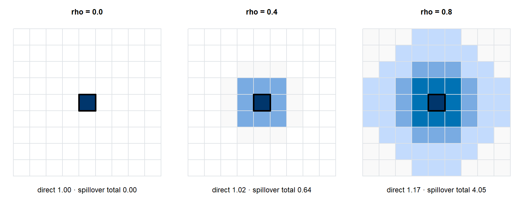
Figure 2: Impacts of raising x by one unit in the centre area (black outline) of a 9 × 9 grid, SAR with β = 1 and row-standardized queen weights. With ρ = 0 only the centre changes (this is OLS). As ρ grows, the change spreads to neighbours and beyond, and feedback raises the centre’s own change (direct impact > 1). The sum of the spillovers can exceed the direct impact.

For SAR, reporting only the raw regression coefficient β can be misleading. Report direct, indirect and total impacts (usually averaged over areas).

Try it. Compute the impact matrix for the toy example, then change ρ.

Watch: Luc Anselin’s lecture on this

▶ Spatial Spillovers: direct, indirect and total impacts

Optional, from the Canvas post. Luc Anselin’s lecture series Applied Spatial Regression Analysis goes beyond STA530 in places.

On the exam, be able to say: Because of feedback, β is not the full effect. Report direct, indirect (spillover) and total impacts; with row-standardized W the total impact is β/(1 − ρ).

3.6 Is a SAR story plausible in epidemiology?

In short. Choose SAR only if it is plausible that outcomes truly affect each other across borders: infections yes, cancer deaths hardly.

The equation may fit the data; the scientific mechanism still needs to make sense.

Outcome	Genuine cross-area outcome process?
Infectious disease	Plausible: cases in one area contribute to transmission into connected areas
Health behaviours	Plausible: social interaction or diffusion can cross administrative boundaries
Cancer mortality	Hard to defend: neighbouring mortality rates do not “cause” one another. Similar rates nearby more likely reflect shared, partly unmeasured exposures → SEM

On the exam, be able to say: SAR fits a genuine cross-area outcome process (infectious disease, diffusion of behaviours). For outcomes such as cancer mortality the mechanism is implausible; correlated errors (SEM) are a better story.

3.7 The spatial error model (SEM) and λ

In short. SEM keeps ordinary regression but lets the errors of neighbouring areas be correlated: something unmeasured and spatially smooth is shared. λ says how strongly.

Think of it as: Neighbours who share the same weather: their outcomes are alike, not because they affect each other, but because of a common cause nobody measured.

\[ y = X\beta + u, \qquad u = \lambda W u + \varepsilon \]

In words: an ordinary regression, except that the error of each area = λ times its neighbours’ errors + fresh noise.

Parameter	Meaning
λ (lambda), error dependence	How strongly the unobserved error process is spatially structured
β, covariates	Regression associations after accounting for correlated errors. Interpreted as in OLS: no spillover impacts
ε, innovation	The remaining independent error

Here neighbouring y values are not on the right-hand side. The dependence sits in the error u.

What creates spatially correlated errors? Unmeasured influences that are similar in nearby areas:

Source	Why it is spatial
Air pollution	Varies smoothly across neighbouring areas but is incompletely measured
Healthcare access	Catchment areas and service environments cross administrative boundaries
Built environment	Unmeasured features of nearby areas resemble one another
SES / context	Area-level social conditions are rarely captured by one covariate

SEM can be viewed as modelling residual spatial structure that X did not explain.

“ρ and λ are the same thing in different models.” Both measure spatial dependence, but in different places. ρ links outcomes (and so changes how β is interpreted, through feedback). λ links errors (β keeps its usual meaning; the dependence mainly affects efficiency and standard errors). Also note: ρ in SAR is unrelated to the ρ mixing parameter in BYM2 (Session 4), which shares only the letter.

On the exam, be able to say: SEM: y = Xβ + u, u = λWu + ε. λ measures spatial dependence in the unexplained part. β is read as in OLS (no spillovers).

3.8 SAR vs SEM: same symptom, different story

In short. Both models handle clustered residuals, but tell different stories: contagion between outcomes (SAR) or a shared hidden cause (SEM). The data alone rarely decide; the mechanism should.

Think of it as: Contagion vs shared weather.

Observed symptom: OLS residuals are spatially autocorrelated. Residual autocorrelation alone does not tell you which story is true.

	Spatial lag (SAR)	Spatial error (SEM)
Equation	y = ρWy + Xβ + ε	y = Xβ + u, u = λWu + ε
Dependence enters through	The outcome	The error process
Link	yᵢ ↔︎ neighbouring y	uᵢ ↔︎ neighbouring u
Mechanism	Interaction, diffusion, feedback / spillovers	Spatially patterned omitted processes
Spatial parameter	ρ	λ
Reading β	Not the full effect: report direct, indirect, total impacts	As in OLS, conditional on X
Epidemiological example	Infectious disease spreading between municipalities	Air quality shared but poorly measured

Figure 3: Causal diagram: an arrow means “directly affects”. Left: SAR, where the outcomes of neighbouring areas affect each other (ρ·Wy). Right: SEM, where there is no arrow between the outcomes; an unmeasured, spatially smooth factor U affects both, so their errors are correlated (λ).

The unexplained part of the outcome is strongly spatially structured

An increase in an area’s outcome raises its neighbours’ outcomes

The covariate effect β has to be split into direct and indirect parts

Sixty percent of the variation in the outcome is caused by geography

λ describes dependence in the error process: the residual (unexplained) variation is spatially correlated. Outcome-to-outcome effects and impacts belong to SAR. λ is not a share of variance explained or caused by space.

Watch: Luc Anselin’s lecture on this

▶ Spatial Process Models: what kind of spatial process each model assumes

Optional, from the Canvas post. Luc Anselin’s lecture series Applied Spatial Regression Analysis goes beyond STA530 in places.

On the exam, be able to say: SAR: dependence in the outcome, ρ, feedback and spillovers. SEM: dependence in the errors, λ, omitted spatially patterned processes. Residual autocorrelation alone does not tell which is true.

3.9 A practical workflow and residual Moran’s I

In short. Fit OLS, check whether the residuals cluster, think about why, compare spatial models, then interpret carefully.

flowchart LR
  A["1 · Fit OLS<br/>scientific model<br/>and covariates"] --> B["2 · Check residuals<br/>map them; test residual<br/>Moran's I"]
  B --> C["3 · Ask why<br/>what mechanism could<br/>create the dependence?"]
  C --> D["4 · Compare models<br/>SAR / SEM + diagnostics;<br/>check residuals again"]
  D --> E["5 · Interpret carefully<br/>impacts for SAR; no causal<br/>language without causal design"]

Workflow: each arrow means “then”. Not causal. From OLS to spatial regression (slide 19).

Diagnostics support reasoning; they do not replace it.

Residual Moran’s I asks: after fitting the model, is there evidence of remaining spatial autocorrelation? If it is significant:

something spatial remains unexplained;
it does not tell SAR from SEM by itself;
it can also reflect other misspecification or heterogeneity.

An important diagnostic goal for the spatial model: substantially reduce unexplained spatial structure (residual Moran’s I near zero after fitting SAR or SEM).

On the exam, be able to say: Residual Moran’s I detects remaining spatial structure but does not distinguish SAR from SEM, and can reflect misspecification. Diagnostics support reasoning; they do not replace it.

3.10 Lagrange multiplier (LM) tests

In short. LM tests ask whether a lag term or an error term would improve the OLS model. The robust versions help when both look significant.

LM tests start from the OLS fit and ask whether adding a spatial component is supported:

Test	Question
LM-lag	Is adding a spatially lagged outcome (ρWy) supported?
LM-error	Is spatial dependence in the errors (λ) supported?
Robust LM-lag / robust LM-error	Each test made robust to the presence of the other kind of dependence. Useful when both simple LM tests are significant

A common reading: if only one simple test is significant, consider that model; if both are, look at the robust versions and see which remains clearly significant.

For this course (slide 21): know what the tests are asking. Do not memorise formulas, and do not treat p-values as the scientific mechanism. Model choice should combine theory, diagnostics and interpretability. The tests are “useful, but not a magic decision tree”.

Watch: Luc Anselin’s lecture on this

▶ Specification Tests: Moran’s I on residuals, LM-lag and LM-error
▶ Robust Tests: the robust LM tests

Optional, from the Canvas post. Luc Anselin’s lecture series Applied Spatial Regression Analysis goes beyond STA530 in places.

On the exam, be able to say: LM-lag tests for a spatially lagged outcome, LM-error for spatially dependent errors; robust versions are used when both are significant. Know what they ask; combine with theory.

3.11 Which model story fits better?

In short. Pick the model whose story matches the process: a shared, poorly measured environment → SEM; an outcome that spreads → SAR.

The slide’s two scenarios:

Scenario	Natural starting model	Why
A. Neighbouring municipalities share an incompletely measured air-quality environment	SEM	The dependence comes from an omitted, spatially smooth exposure: correlated errors
B. An infectious outcome diffuses through movement between connected municipalities	SAR may be plausible	Outcomes in one area directly affect outcomes in connected areas

Real analyses can be less clean. The point is to articulate the assumed process.

Spatial lag (SAR), because uptake itself spreads between areas

Spatial error (SEM), because uptake is shaped by unmeasured factors

OLS, because spatial dependence never affects the estimated β

A model with no W, since diffusion is not a geographic process

Social diffusion of behaviour is an outcome-to-outcome process, which is what ρWy represents. With SAR, remember to report direct and indirect (spillover) impacts instead of β alone.

On the exam, be able to say: Shared incompletely measured air quality → SEM; infectious diffusion between connected areas → SAR. The point is to state the assumed process.

3.12 Deliberately not covered in STA530

In short. Estimation methods and more advanced spatial models are outside the course.

The slides list what the session leaves out:

maximum-likelihood derivations;
instrumental variables / generalized method of moments (GMM) estimation;
higher-order spatial models;
spatial Durbin and SLX models (which add WX, the neighbours’ covariates);
geographically weighted regression (GWR) and other spatial heterogeneity models.

The stated goal: understand what spatial dependence means, recognize basic models, and interpret them responsibly — not become spatial econometricians in 90 minutes.

Watch: Luc Anselin’s lecture on this

▶ Spatial Durbin Model
▶ Principles of Maximum Likelihood Estimation
▶ ML Estimation of Spatial Lag Model
▶ ML Estimation Spatial Error Model
▶ 2SLS
▶ IV Estimation of Spatial Lag Model
▶ GMM Estimation Principle
▶ GMM Estimation of Spatial Error Model

These cover exactly what STA530 leaves out (estimation and the Durbin model). Not needed for the course.

3.13 Take-home messages and key questions

Check geography after regression. Spatial structure can remain after covariate adjustment.
SAR and SEM encode different mechanisms: outcome feedback versus spatially correlated errors.
SAR changes interpretation: direct and indirect impacts matter because of feedback.
Diagnostics are evidence, not answers: use residual checks and tests together with scientific reasoning.

Why is β in a SAR model not the full effect of x?

Because y appears on both sides. A change in x in one area changes y there, which changes neighbours’ y through ρW, which feeds back. The total effect is captured by (I − ρW)⁻¹β; with row-standardized W the total impact is β/(1 − ρ), larger than β when ρ > 0.

Residual Moran’s I is significant. Why can you not conclude that SAR is the right model?

Because both SAR (outcome dependence) and SEM (error dependence) produce autocorrelated OLS residuals, and so can misspecification or spatial heterogeneity. The diagnostic says something spatial is unexplained, not which mechanism. Theory, LM tests and interpretability have to be combined.

What does ρ represent in SAR, and λ in SEM?

ρ is the strength of dependence between an area’s outcome and its neighbours’ outcomes (through Wy). λ is the strength of spatial dependence in the error process: how spatially structured the unexplained part is.

Why might OLS standard errors be wrong with positively autocorrelated residuals?

OLS treats every area as an independent piece of information. If neighbouring residuals are alike, the effective amount of information is smaller than n, so the true sampling variability of β̂ is larger than OLS reports: standard errors too small, confidence intervals too narrow, p-values too small.