Session 2 — Disease Mapping and Spatial Patterns

Choropleth classification · extreme value maps · counts vs rates · variance instability · SMR · Empirical Bayes smoothing · spatial weights · Moran’s I · LISA

Session 2 moves from making maps to evaluating spatial patterns. It has two halves.

The first half is about maps of disease. How you classify a variable into colours changes what the reader sees, and crude rates from small populations are unstable: an area with 50 inhabitants can show a very high or very low rate purely by chance. The standardized mortality ratio (SMR) and Empirical Bayes smoothing are the first tools for this.

The second half formalises Tobler’s law. To ask whether nearby areas are similar, you first have to define who is a neighbour (a spatial weights matrix). Then Moran’s I measures global spatial autocorrelation, and local Moran’s I (LISA) says where the clusters and outliers are.

Sources and session

Slides: “session_2_v0.pdf” (Qinyun Lin, 6 October 2026, 15:15–17:00). Several figures on the slides come from the GeoDa workbook, Anselin’s course material and the Axis Maps guide to data classification.

Learning objectives (Canvas post): after this session you should be able to

explain why mapping counts and crude rates can produce different spatial patterns;
explain why estimates from areas with small populations can be unstable;
describe different ways of defining spatial neighbours;
interpret positive and negative spatial autocorrelation;
explain the basic idea of Moran’s I;
distinguish between global and local spatial autocorrelation.

Topics that match an objective carry 🎯.

Before you start: three ideas from earlier courses

Quartiles and the IQR. Q1 and Q3 cut off the lowest and highest 25%. IQR = Q3 − Q1. A box plot calls values beyond Q1 − 1.5·IQR or Q3 + 1.5·IQR outliers.

Variance of a proportion. If a proportion is estimated from n people with true probability π, its variance is π(1 − π)/n. Halving n doubles the variance.

What a p-value means. The probability, if the null hypothesis were true, of a test statistic at least as extreme as the one observed. It is not the probability that the null hypothesis is true. The slides ask you to recall this before the Moran’s I test.

2.1 Thematic (choropleth) maps and classification methods

In short. A choropleth map colours areas by their value. Where you put the colour boundaries decides whether the same data look calm or alarming.

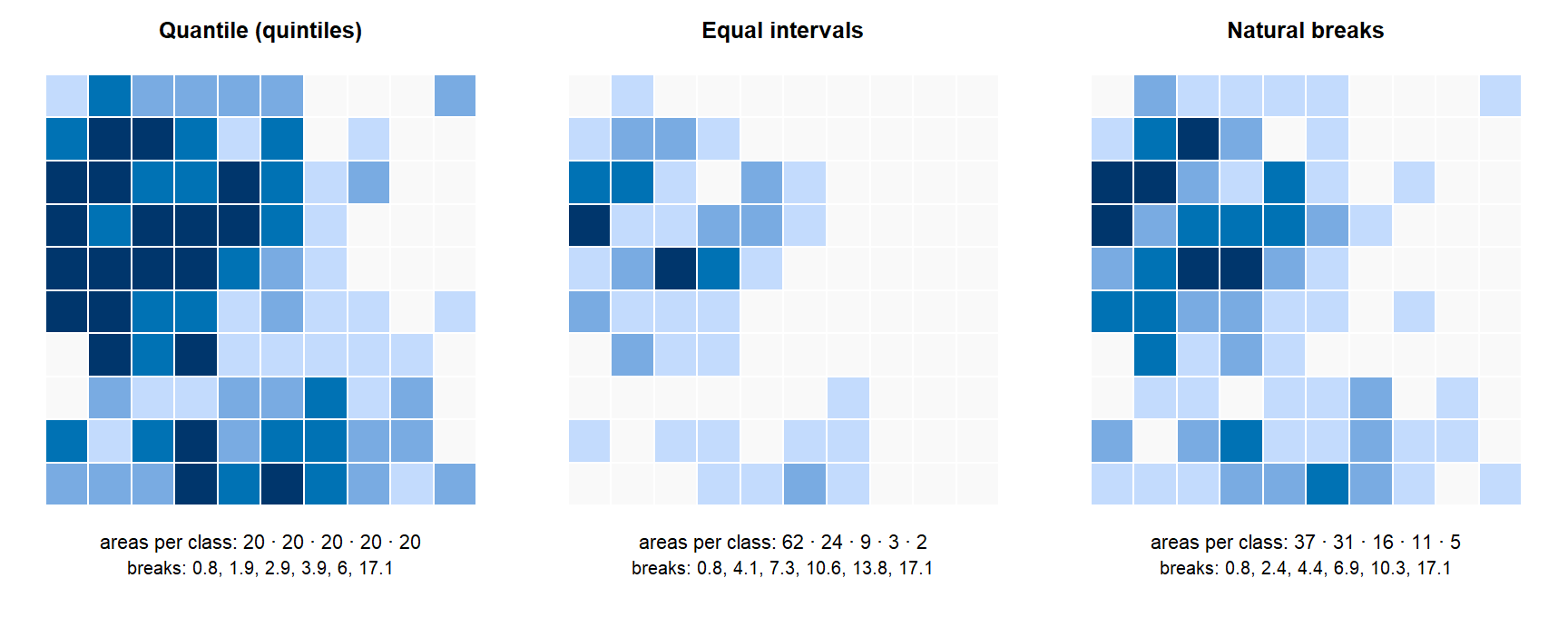
A thematic or choropleth map shows values with colours or patterns inside geographic areas. Two choices change the picture: the classification method (where the class boundaries go) and the number of classes.

Method	How the class breaks are chosen	Strength	Weakness
Quantile	Each class has the same number of areas (3 = tertiles, 4 = quartiles, 5 = quintiles)	Every colour is used equally; good for ranking	Very different values can share a class; close values can be split
Natural breaks (Jenks)	Breaks minimise variation within classes and maximise differences between them	Follows gaps in the data	Classes can hold very unequal numbers of areas; hard to compare maps
Equal intervals	The range is cut into classes of equal width	Easy to read	One extreme value can push most areas into one class
Manual intervals	You choose meaningful cut-offs (for example clinical thresholds)	Interpretable	Needs justification
Standard deviation	Values are expressed in SD units from the mean	Shows how far from average; spots outliers	Assumes a roughly symmetric distribution

Figure 1: The same skewed rates on a 10 × 10 grid with three classification methods and five classes. Quantiles fill every class equally and make the map look busy; equal intervals put most areas in the lowest class; natural breaks follow gaps in the values. Same data, three impressions. (Natural breaks approximated here with one-dimensional k-means.)

There is no universally best method. It depends on the distribution of the data, the purpose of the map and the comparison you want the reader to make.

Read more: Axis Maps, Data classification (source of the classification figures on the slides).

Almost every area in the lowest class, a few in the top ones

Each class holding the same number of areas, as in quintiles

Classes chosen at the natural gaps between groups of values

All areas coloured by how many SDs they lie from the mean

Equal intervals split the range evenly. A few extreme values stretch the range, so most areas fall in the bottom interval. A quantile map would instead force equal counts per class.

On the exam, be able to say: Classification methods: quantile (equal number of areas per class), equal interval, natural breaks (minimise within-class variation), standard deviation, manual. No method is best in general; it depends on the data and the purpose.

2.2 Extreme value maps: percentile, box and standard deviation maps

In short. Extreme-value maps are built to make outliers stand out. A box map flags areas outside the box-plot fences; a percentile map always shows the top and bottom 1%.

Extreme value maps are designed to highlight outliers rather than show the whole distribution evenly.

Map	Classes
Percentile map	Fixed percentile cut-offs: < 1%, 1–10%, 10–50%, 50–90%, 90–99%, > 99%
Box map	The box plot’s categories: lower outlier, < 25%, 25–50%, 50–75%, > 75%, upper outlier
Standard deviation map	Classes in SD units around the mean

Box map fences. Lower bound LB = Q1 − hinge × IQR, upper bound UB = Q3 + hinge × IQR.

	Hinge = 1.5	Hinge = 3
Q1, Q3, IQR (rent example on the slide)	1000, 1362.5, 362.5	same
LB	1000 − 1.5 × 362.5 = 456.25	1000 − 3 × 362.5 = −87.5
UB	1362.5 + 1.5 × 362.5 = 1906.25	1362.5 + 3 × 362.5 = 2450
Effect	More outliers flagged	Fewer and more extreme outliers flagged

The slide’s question: which map is the box map and which is the percentile map? Read the legend. A box map’s legend has “Lower outlier”, “< 25%”, “25–50%”, “50–75%”, “> 75%”, “Upper outlier”, with the outlier classes holding however many areas lie beyond the fences (possibly none). A percentile map’s legend has the fixed bins < 1%, 1–10%, 10–50%, 50–90%, 90–99%, > 99%, so its extreme classes always hold about 1% of areas each.

On the exam, be able to say: Box map fences: Q1 − hinge·IQR and Q3 + hinge·IQR; hinge 3 flags fewer, more extreme outliers than hinge 1.5.

2.3 Mapping categorical variables and co-location

In short. Each category gets its own colour. A co-location map shows where two characteristics occur in the same place.

A unique value map gives each category its own colour (for example urban / suburban / rural).

A co-location map extends it to show where several characteristics overlap. The slide’s example marked US counties with both persistently high COVID-19 mortality and a high population share of a particular racial/ethnic group, so you can see where the two coincide. Co-location shows overlap, not cause.

2.4 Counts vs rates, and the problem of variance instability

In short. Counts mostly show where people live; rates show risk. But rates from small populations jump around by chance, so the most extreme rates are often just the smallest areas.

Think of it as: A basketball player who scores 2 of 2 shots has 100%, yet you would trust 450 of 500 (90%) much more.

Two kinds of variables behave differently on a map:

	Spatially extensive	Spatially intensive
Depends on population size?	Yes	No, standardized by population
Example	Number of cases or deaths	Rate or risk: cases per population
What a map shows	Mostly where people live	Where the risk is high

Mapping counts therefore mostly reproduces a population map: big cities have the most cases. Crude rates fix this, but bring a new problem.

Variance instability. For area i with observed cases Oᵢ and population at risk Pᵢ, the crude risk is rᵢ = Oᵢ / Pᵢ. If the underlying risk is πᵢ,

\[ \operatorname{Var}(r_i) = \frac{\pi_i (1 - \pi_i)}{P_i}. \]

In words: the uncertainty of a crude rate is the true risk times one minus it, divided by the population: the fewer people, the noisier the rate.

Small Pᵢ → large variance → unstable crude estimates. Areas with small populations show very high or very low crude rates simply because of sampling variability. This motivates smoothing.

The slide’s question: with the same underlying πᵢ, which area has the more variable observed risk, Pᵢ = 100 or Pᵢ = 10,000? Pᵢ = 100: its variance is 100 times larger (its standard deviation 10 times larger).

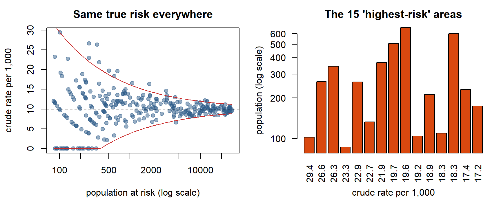
Simulated: 300 areas that all share the same true risk of 1%. Left: crude rates against population size. The most extreme rates, both high and low, all belong to small areas, a ‘funnel’. Right: the map-maker’s view, the 15 highest crude rates; nearly all are small areas with no real excess risk.

Small populations give unstable rates that scatter in both directions

Rural areas have a genuinely more extreme mix of cancer risk factors

Counts were mapped instead of rates, so population size dominates

The classification method put rural areas in the extreme classes

Extremes in both directions in small areas is the signature of variance instability. A real rural risk factor would push rates one way, not both ways.

On the exam, be able to say: Counts are spatially extensive (depend on population size); rates are intensive. Var(rᵢ) = πᵢ(1 − πᵢ)/Pᵢ, so small populations give unstable crude rates: variance instability. This motivates smoothing.

2.5 Comparing areas with the SMR (excess risk)

In short. The SMR compares what happened with what would have happened if the area had the reference risk: SMR = observed ÷ expected.

An excess risk map compares each area’s rate with a reference risk (national or regional). The reference risk is estimated from all observations pooled:

\[ \hat\pi = \frac{\sum_{i=1}^{n} O_i}{\sum_{i=1}^{n} P_i} = \frac{\text{total events}}{\text{total population at risk}}. \]

Expected count and standardized mortality ratio (SMR):

\[ E_i = \hat\pi \times P_i, \qquad \text{SMR}_i = \frac{O_i}{E_i} = \frac{O_i}{\hat\pi P_i} = \frac{r_i}{\hat\pi}. \]

In words: expected cases = the reference risk times the area’s population; the SMR is observed divided by expected.

The slide’s two questions:

Is π̂ equal to the average of all rates? No. π̂ is a population-weighted average: total events over total population. The simple mean of the area rates gives every area the same weight, so a few small areas with extreme rates can pull it far away. They coincide only if all areas have the same population.
How to interpret SMRᵢ > 1? Area i had more events than expected if the reference risk applied there. SMR = 1.3 means 30% more than expected. It is not, on its own, evidence of a real excess: a small Eᵢ makes the SMR unstable (Session 4).

Slide practice. Overall cancer risk 10%. Area A has 1,000 residents at risk; 20 get cancer.

Approach	Calculation	SMR
1: expected count	E = 1000 × 10% = 100; SMR = 20 / 100	0.2
2: rate ratio	crude rate = 20 / 1000 = 2%; SMR = 2% / 10%	0.2

Area A has 80% fewer cases than expected.

Expected counts can also use stratum-specific reference risks (by age and sex): indirect standardization, worked through in Session 4.

On the exam, be able to say: Eᵢ = π̂ × Pᵢ with π̂ = total events / total population (a population-weighted average, not the mean of the rates). SMR = O/E; SMR > 1 means more events than expected.

2.6 Empirical Bayes smoothing

In short. EB smoothing pulls each crude rate toward the overall rate, more strongly the smaller the population. Reliable areas keep their own rate; noisy ones borrow from the average.

Think of it as: Restaurant ratings. A 5.0 from 3 reviews is less convincing than a 4.6 from 3,000, so a sensible guess for the first restaurant moves toward the typical rating.

Idea: replace each crude rate by a weighted average of the area’s own crude rate and the overall (reference) rate:

\[ \hat\pi_i^{EB} = w_i\, r_i + (1 - w_i)\, \theta, \qquad w_i = \frac{\sigma^2}{\sigma^2 + \mu / P_i}. \]

In words: the smoothed rate is a weighted average of the area’s own rate and the reference rate. The weight compares real differences between areas (σ²) with noise (μ/Pᵢ): little noise → trust the area, much noise → trust the reference.

Symbol	Meaning
rᵢ	Crude rate in area i
θ (= μ)	Prior estimate: the reference rate (overall average or another standard)
σ²	Variance of the true rates between areas (how much real variation there is)
μ / Pᵢ	Approximately the sampling variance of rᵢ: large when Pᵢ is small
wᵢ	Weight on the area’s own data, between 0 and 1

Reading the weight. wᵢ compares real between-area variation (σ²) with noise (μ/Pᵢ):

large, informative area: μ/Pᵢ is tiny, wᵢ ≈ 1 → little shrinkage, the area keeps its own rate;
small, uninformative area: μ/Pᵢ is large, wᵢ is small → strong shrinkage toward the reference rate.

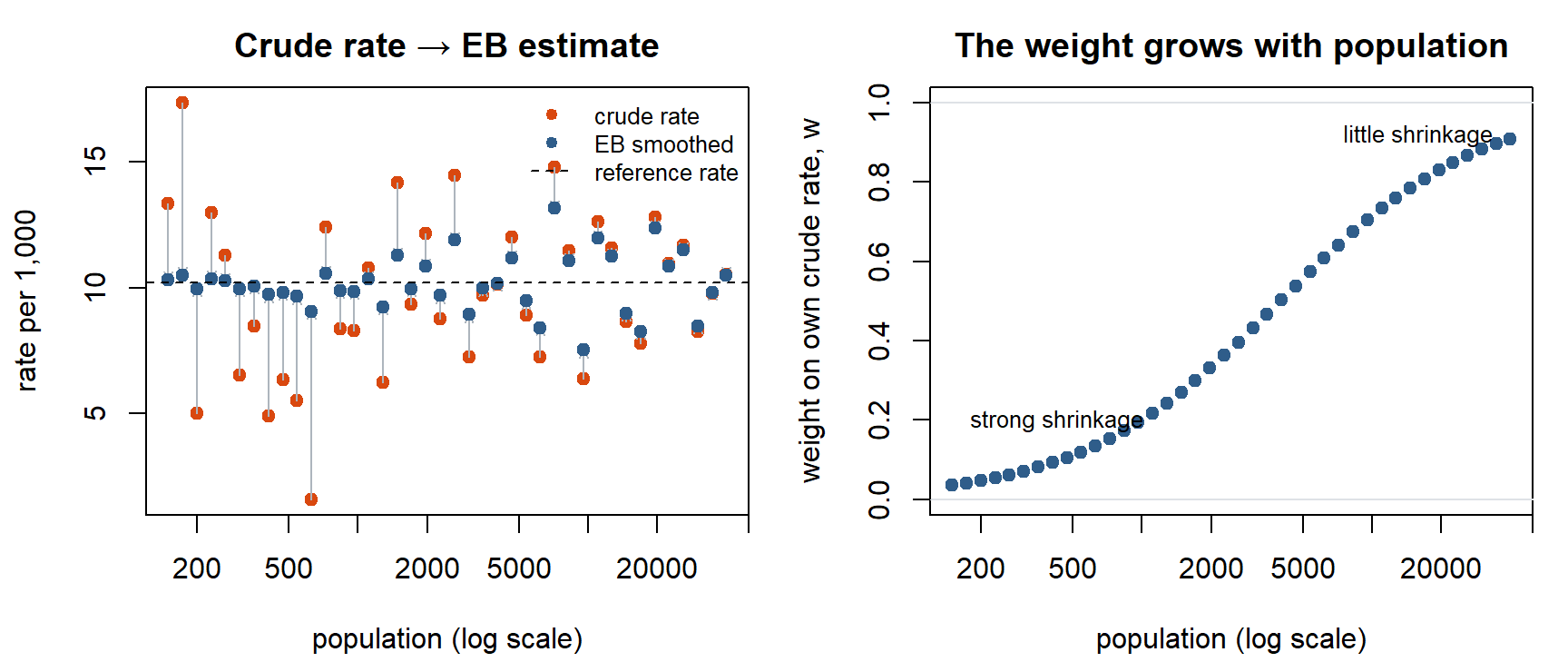
Figure 2: Empirical Bayes smoothing, simulated: 40 areas whose true risks vary moderately around 1%. Left: each grey line shows how far a crude rate (orange) moves to its EB estimate (blue). Small areas are pulled almost all the way to the reference rate; large areas barely move. Right: the weight w on the area’s own rate grows with population.

EB smoothing reduces the influence of unstable extreme estimates from small populations.

“Empirical Bayes is a Bayesian method.” Not quite. The prior (θ and σ²) is estimated from the same data rather than specified beforehand, and the method produces point estimates without a full posterior distribution. It borrows the Bayesian idea of shrinkage. (The same trick is used in moderated t-tests for gene expression: small samples get their variance shrunk.) Fully Bayesian disease mapping is Session 4.

Three maps of the same data (slides 17–18): a raw rate map, an excess risk map (SMR) and an EB smoothed map can look quite different. In the raw and excess risk box maps, small areas often appear as outliers; after EB smoothing, many of them move back toward the middle and the remaining outliers are more trustworthy.

When to use EB smoothing

When areas differ a lot in population size and the goal is a map of risk that is not dominated by small-area noise. It is quick and needs no model fitting.

Limitations

It ignores geography: every area is shrunk toward the same global mean, not toward its neighbours (spatial EB versions exist). It gives no full uncertainty for each area. A genuinely high-risk small area is pulled toward the mean too, so real local excesses can be hidden.

On the exam, be able to say: EB estimate = wᵢ·rᵢ + (1 − wᵢ)·θ with wᵢ = σ²/(σ² + μ/Pᵢ). Small areas get small weights (strong shrinkage), large areas keep their own rate. The prior is estimated from the data, so it is not fully Bayesian.

2.7 Spatial autocorrelation and the null of spatial randomness

In short. Spatial autocorrelation asks: are nearby areas more alike than they would be if the values had been scattered at random over the map?

Think of it as: Shuffle the map like a deck of cards many times. If the real map is more clustered than almost all shuffled maps, the pattern is not chance.

Spatial autocorrelation formalises Tobler’s law: the correlation of a variable with itself across space.

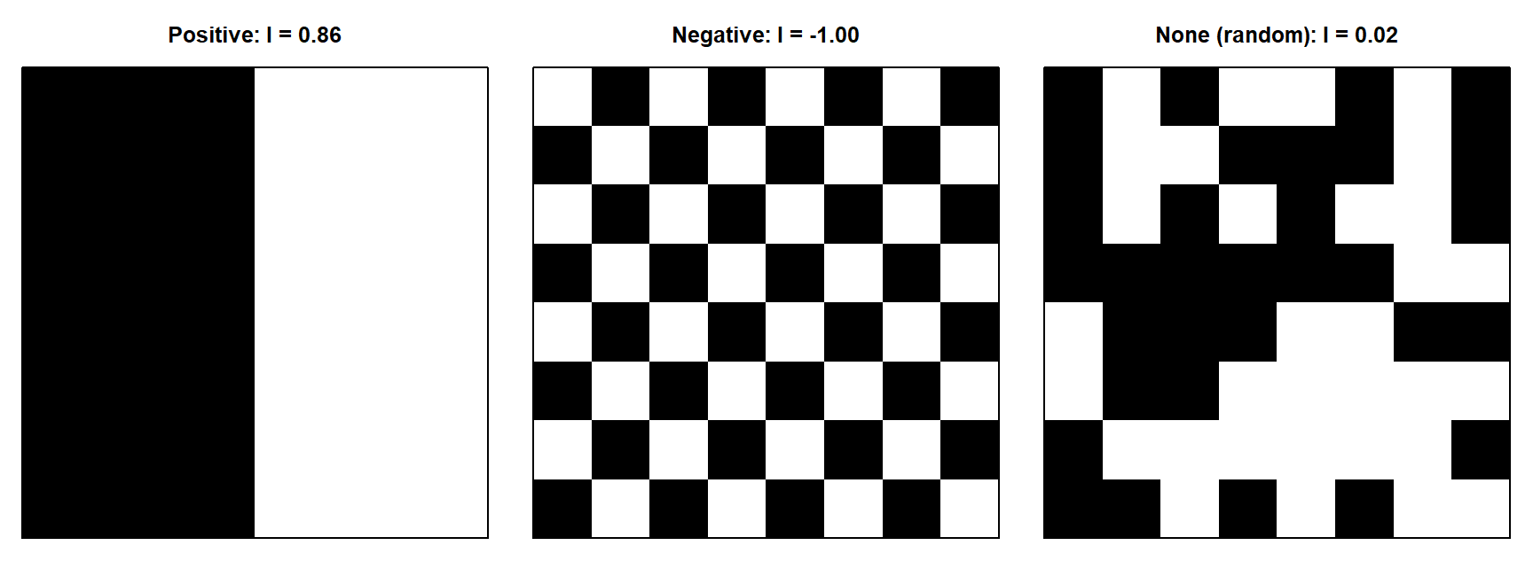
Three 8 × 8 patterns with the same number of black and white cells (as on slide 20, after O’Sullivan and Unwin 2002). Moran’s I uses binary rook weights.

Testing. A test statistic summarises the data and is compared with its distribution under the null hypothesis. For spatial autocorrelation the null is spatial randomness: the observed values are not systematically associated with their locations. Any arrangement of the values over the map would be equally likely.

That suggests a direct test: randomly permute (reshuffle) the values over the locations many times, compute the statistic each time, and see where the observed value falls.

To measure autocorrelation you need two kinds of similarity at once:

attribute similarity: are two values alike? (for Moran’s I, the product of deviations from the mean, zᵢzⱼ);
locational similarity: are the two areas neighbours? (the spatial weight wᵢⱼ).

On the exam, be able to say: Positive autocorrelation: similar values cluster; negative: neighbours differ (checkerboard). The null hypothesis is spatial randomness, tested by comparing with random permutations.

2.8 Spatial weights: contiguity (rook and queen)

In short. Before you can say “neighbours are alike”, you must decide who counts as a neighbour. Rook: a shared border; queen: a shared border or corner. The weights matrix W records the choice.

Before testing for autocorrelation you must define neighbours. A spatial weights matrix W records, for every pair of areas, whether (or how strongly) they are neighbours: wᵢⱼ = 1 if i and j are neighbours, 0 otherwise, and wᵢᵢ = 0. Choosing W means thinking about how far an influence can reach.

3 × 3 grid, rook contiguity (from the slide). Areas are numbered row by row:

1	2	3
4	5	6
7	8	9

	1	2	3	4	5	6	7	8	9
1	0	1	0	1	0	0	0	0	0
2	1	0	1	0	1	0	0	0	0
3	0	1	0	0	0	1	0	0	0
4	1	0	0	0	1	0	1	0	0
5	0	1	0	1	0	1	0	1	0
6	0	0	1	0	1	0	0	0	1
7	0	0	0	1	0	0	0	1	0
8	0	0	0	0	1	0	1	0	1
9	0	0	0	0	0	1	0	1	0

The matrix is symmetric, the diagonal is 0, the centre (5) has 4 neighbours and corners have 2.

	Rook contiguity	Queen contiguity
Neighbours if they share	A boundary (edge), not just a corner	A boundary or a corner
Number of neighbours	Fewer	More (includes all rook neighbours)
Higher orders	Yes	Yes
Islands / unconnected areas	Not connected	Not connected

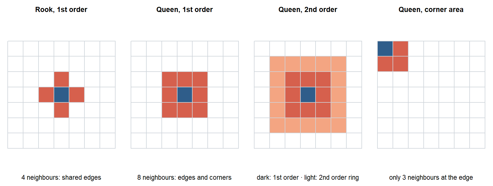
Figure 3: Neighbour definitions on a regular grid. The blue area is the target; red cells are its neighbours. An edge or corner area has fewer neighbours than an interior one.

The slide’s question: if both are first order, which has more neighbours? Queen, because it adds the corner (diagonal) neighbours. On a regular grid, an interior cell has 4 rook and 8 queen neighbours.

Higher order. Second-order neighbours are neighbours of neighbours (the next ring out). Software may or may not include the first order as well; the slide’s figure shows the target county, its first-order queen ring and the second-order ring. Same area, different W, different results.

Row standardization. Dividing each row by its row sum makes each row sum to 1, so wᵢⱼ = 1/nᵢ. Then Σⱼ wᵢⱼ xⱼ is the average of the neighbours’ values, the spatial lag. This comes back in Moran’s scatter plot, the SAR model and the CAR prior.

On the exam, be able to say: W has wᵢⱼ = 1 if i and j are neighbours, else 0, with zeros on the diagonal. Queen contiguity gives at least as many neighbours as rook. Higher orders are neighbours of neighbours. Row standardization makes Wy the neighbour average.

2.9 Spatial weights: distance bands and k-nearest neighbours

In short. Neighbours can also be defined by distance: everyone within a set distance (distance band), or each area’s k nearest. KNN guarantees that everyone has neighbours, but the relation is not symmetric.

Think of it as: KNN is like “your four closest friends”: you may be on their list, or not.

Distance-based weights use the distance between points (or area centroids).

Distance metrics

Metric	Formula / idea	Use when
Euclidean (straight line)	\(d_{ij} = \sqrt{(x_i - x_j)^2 + (y_i - y_j)^2}\)	Coordinates are projected (on a plane, in metres)
Great circle / arc distance	Distance along the Earth’s curved surface	Unprojected longitude/latitude

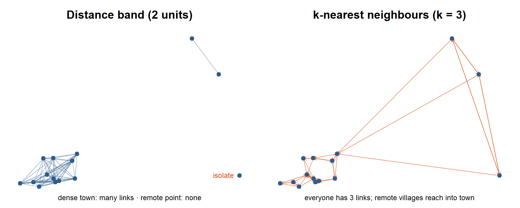
Distance-band weights. i and j are neighbours whenever j is within a critical distance of i. The result is symmetric. To avoid isolates, the threshold is often set to the largest nearest-neighbour distance (so every area has at least one neighbour), but then areas in dense clusters can get very many neighbours.

Isolates are areas with no neighbours. They drop out of all spatial analyses (autocorrelation tests, spatial regression), although they are fine in non-spatial analysis. Ignoring them is a problem for spatially lagged variables and local statistics.

k-nearest-neighbour (KNN) weights. Choose k (say 4); each area gets its k nearest neighbours (by centroid distance).

Connects every area: no isolates.
Not symmetric: B can be among A’s 4 nearest without A being among B’s 4 nearest (B may sit in a dense cluster). It can be made symmetric, for example \(w^*_{ij} = (w_{ij} + w_{ji})/2\).
Ties: several areas at the same distance; choose randomly or include all.

	Contiguity	Distance band	KNN
Symmetric?	Yes	Yes	No (unless symmetrized)
Isolates possible?	Yes (islands)	Yes, unless threshold ≥ max nearest-neighbour distance	No
Number of neighbours	Varies	Varies a lot (dense vs sparse areas)	Exactly k for every area

Figure 4: The same 15 points with two distance-based definitions. Left: a 2-unit distance band links the dense town heavily and leaves a remote point as an isolate. Right: with k = 3 nearest neighbours every point has exactly three links (arrows), even remote villages, and the links are not symmetric: a village points into town, but the town points do not point back.

k-nearest-neighbour weights, for example k = 4

First-order rook contiguity weights between areas

First-order queen contiguity weights between areas

A distance band shorter than the largest nearest-neighbour gap

Contiguity weights leave islands without neighbours, and a distance band only connects everyone if its threshold is at least the largest nearest-neighbour distance. KNN always gives each area exactly k neighbours.

On the exam, be able to say: Distance band: symmetric, but dense areas get many neighbours and isolates are possible. KNN: exactly k neighbours each, no isolates, not symmetric, ties possible. Use Euclidean distance only for projected coordinates.

2.10 Describing a weights matrix: connectivity histogram and graph

In short. Two quick checks of a weights matrix: how many neighbours each area has (histogram) and a picture of the links (graph).

Two diagnostics show what a weights matrix looks like:

Connectivity histogram: how many areas have 1, 2, 3, … neighbours.
Connectivity graph: a line between the centroids of every pair of neighbours.

The slides’ questions:

What does the histogram look like with KNN weights? A single bar at k: every area has exactly k neighbours. (If you symmetrize the KNN matrix, some areas gain neighbours and the histogram spreads to the right of k.)

Which graph suggests KNN and which suggests a distance band? With a distance band, dense areas (cities) have very many links, sparse areas have few, and isolated points may have none. With KNN, every point has the same number of links, even remote points, which reach out with long lines to their nearest neighbours.

Read more: GeoDa workbook, Distance-based spatial weights (source of the connectivity histogram and graph on the slides).

On the exam, be able to say: With KNN the connectivity histogram is a single bar at k. With a distance band, dense areas have many links and remote points may have none.

2.11 Global Moran’s I

In short. Moran’s I is one number for the whole map: positive when neighbours are alike, negative when they differ, close to zero when there is no pattern. Whether it is unusual is judged against shuffled maps.

\[ I = \frac{\sum_{i=1}^{n}\sum_{j=1}^{n} w_{ij}\, z_i z_j \,/\, S_0}{\sum_{i=1}^{n} z_i^2 \,/\, n}, \qquad z_i = x_i - \bar x, \qquad S_0 = \sum_i\sum_j w_{ij}. \]

In words: for every pair of neighbours, multiply how far each is from the mean; average these products over all neighbour pairs and divide by the overall variance. Mostly positive products (high next to high, low next to low) → I > 0.

Reading it. The numerator is a cross-product between each value and its neighbours (attribute similarity × locational similarity), averaged over all neighbour pairs. The denominator is the variance. So Moran’s I is like a correlation between a variable and its spatial lag.

zᵢ and its neighbours’ zⱼ	Product zᵢzⱼ	Contribution
Both above the mean (high next to high)	+	Positive
Both below the mean (low next to low)	+	Positive
One above, one below (high next to low)	−	Negative

Inference. H₀: spatial randomness. Two ways to judge whether the observed I is unusual:

Approach	How	Pros / cons
Analytical	Normal approximation with the theoretical mean and variance of I	Fast; sensitive to distributional assumptions
Permutation (computational)	Randomly reshuffle the values over the areas many times, compute I each time, compare the observed I with this reference distribution → pseudo p-value	More robust; limited to the actual sample. More permutations (999 rather than 99) give more stable results

Moran’s I depends on the weights: the same data with another W give another I.

“Under the null hypothesis Moran’s I equals 0.” Its expected value under spatial randomness is \(E[I] = -1/(n-1)\), slightly negative. For 100 areas that is about −0.01, so in practice “about 0”. With very few areas the difference matters.

The pseudo p-value from R permutations is (number of permuted I ≥ observed I, plus 1) / (R + 1). With 999 permutations the smallest possible value is 1/1000 = 0.001.

Try it: the permutation test in your browser. The code builds an 8 × 8 grid with a smooth gradient plus noise, computes Moran’s I with rook weights, and compares it with 999 random reshuffles. Change trend_strength to 0 and run again.

On the exam, be able to say: Moran’s I is a cross-product of deviations between neighbours, scaled by the variance. It is tested against spatial randomness, analytically or by permutation (pseudo p-value). It depends on W. E[I] = −1/(n − 1) under the null.

2.12 The Moran scatter plot

In short. Plot each area’s value against the average of its neighbours. The slope of the line is Moran’s I, and the four quadrants show clusters (HH, LL) and outliers (HL, LH).

With row-standardized weights (S₀ = n), Moran’s I simplifies to

\[ I = \frac{\sum_i z_i \cdot \left(\sum_j w_{ij} z_j\right)}{\sum_i z_i^2}, \]

which is the slope of a regression line of the spatial lag Σⱼwᵢⱼzⱼ on zᵢ. The Moran scatter plot:

x-axis: each area’s own (standardized) value;
y-axis: its spatially lagged value (the average of its neighbours);
slope = Moran’s I.

The four quadrants classify areas:

Quadrant	Own value	Neighbours	Type
Upper right	High	High	High-High: cluster (hot spot)
Lower left	Low	Low	Low-Low: cluster (cold spot)
Lower right	High	Low	High-Low: spatial outlier
Upper left	Low	High	Low-High: spatial outlier

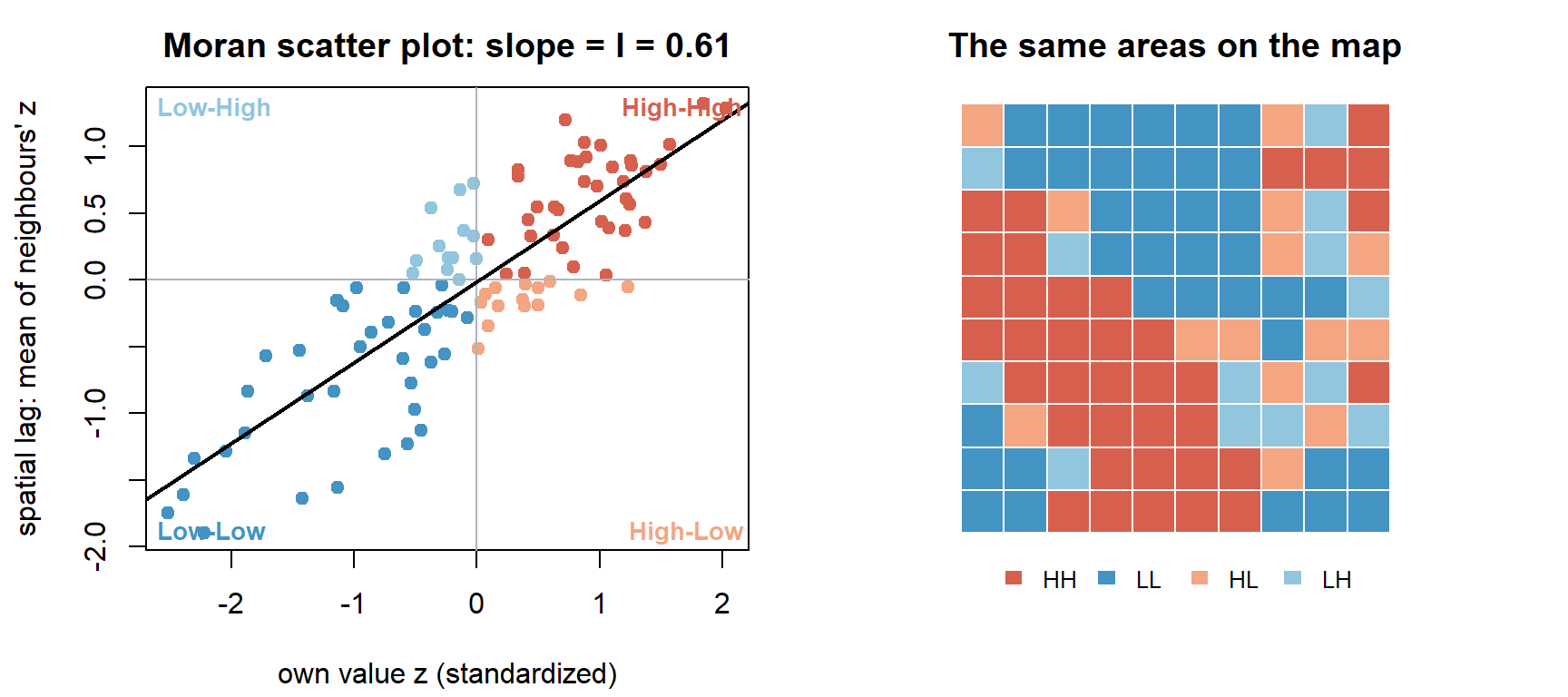
Figure 5: Moran scatter plot for a simulated 10 × 10 map (row-standardized queen weights). Each point is one area: its own standardized value against the average of its neighbours. The slope of the line is Moran’s I. Right: the quadrant of each area drawn back on the map. This is not yet a significance test; LISA (2.13) adds that.

“High” and “low” are relative to the mean.

The slides’ questions. Spatial clusters (HH, LL): positive autocorrelation. Spatial outliers (HL, LH): negative autocorrelation (the area is unlike its neighbours).

On the exam, be able to say: Moran scatter plot: x = own value, y = spatial lag. Slope = Moran’s I (row-standardized W). HH/LL are positive association (clusters), HL/LH negative (outliers), relative to the mean.

2.13 Local spatial autocorrelation: LISA and local Moran’s I

In short. Global Moran’s I says whether there is clustering; LISA says where. Each area gets its own statistic and p-value, and significant areas are labelled HH, LL, HL or LH.

	Global	Local
Question	Is there spatial clustering?	Where, and what type?
Output	One number for the whole map	One statistic and one p-value per area
Measures	Moran’s I (Geary’s C)	LISA, for example local Moran’s I; local Geary
Finds	Overall clustering	Hot spots, cold spots and spatial outliers

Deeper: the formal definition of a LISA

LISA (local indicator of spatial association, Anselin 1995) must:

give a statistic for each location with an assessment of significance;
be such that the sum of the local statistics is proportional to the global statistic.

Generic local form Σⱼ wᵢⱼ f(xᵢ, xⱼ); generic global form Σᵢ Σⱼ wᵢⱼ f(xᵢ, xⱼ).

Local Moran’s I:

\[ I_i = \frac{z_i \sum_j w_{ij} z_j}{\sum_i z_i^2 } , \]

In words: an area’s own deviation from the mean times its neighbours’ deviations. Large and positive = the area and its neighbours are on the same side of the mean (a cluster); negative = opposite sides (an outlier).

the area’s own deviation times the weighted sum of its neighbours’ deviations. Global Moran’s I corresponds to the average of the local statistics (their sum is proportional to the global I).

Significance by conditional permutation. As for the global test, except that zᵢ is held fixed at location i and only the other values are reshuffled over its neighbours. This gives a pseudo p-value for each area.

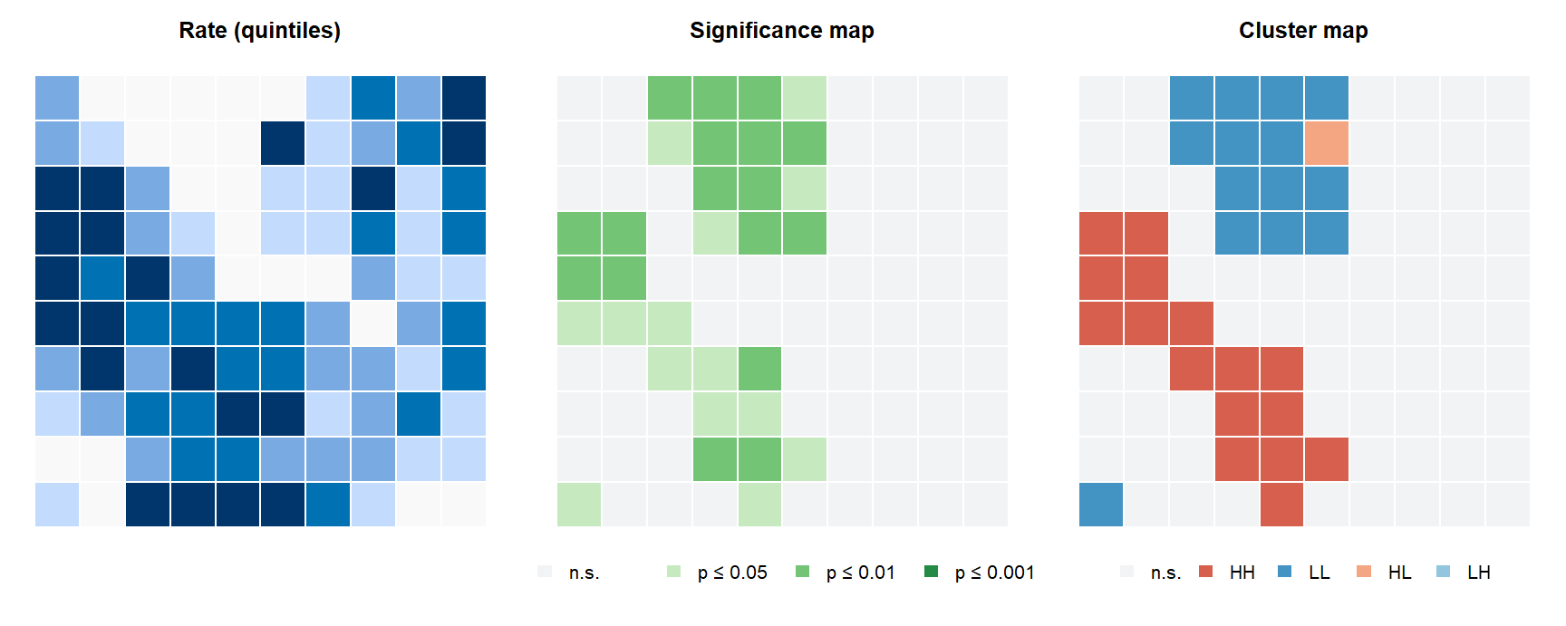
Two maps come out of a LISA analysis:

a significance map: areas coloured by pseudo p-value (0.05, 0.01, 0.001);
a cluster map: the significant areas coloured by type: High-High and Low-Low clusters, High-Low and Low-High outliers.

Figure 6: LISA, simulated. Left: the rate map. Middle: the significance map, pseudo p-values from conditional permutation. Right: the cluster map, the significant areas coloured by type. The one HL area is an odd high value placed inside a low region: a spatial outlier.

Interpreting a cluster map

“High” and “low” are relative to the mean of the variable. A High-High area is significant together with its neighbours: the cluster is the core area and its neighbours, not just the coloured area. With many areas, some will be significant at 0.05 by chance (multiple testing); stricter cut-offs (0.01, 0.001) or false discovery rate adjustments are often used. And LISA on raw rates inherits variance instability: small areas can produce spurious clusters.

Its value is below the mean while its neighbours’ values are above it

Its value is below the mean and so are those of its neighbours

Its value is above the mean while its neighbours’ are below it

It belongs to a cold spot that is surrounded by a hot spot

The first word describes the area itself, the second its neighbours (spatial lag), both relative to the mean. Low-High is a spatial outlier: a low value among high neighbours, which is negative local autocorrelation.

When to use global vs local statistics

Global Moran’s I first, to ask whether there is clustering at all. LISA when you need to locate clusters and outliers, for example for surveillance or to target resources. Choose and report W, and check robustness to another W.

Read more: GeoDa workbook, Local spatial autocorrelation (source of the significance and cluster maps on the slides).

On the exam, be able to say: LISA gives a local statistic with significance for each location, and the local statistics sum (proportionally) to the global one. Local Moran’s I is tested by conditional permutation; results are shown in significance and cluster maps.

2.14 Session summary and key questions

flowchart LR
  A["Map counts"] -->|"population dominates"| B["Map crude rates"]
  B -->|"small areas unstable"| C["SMR / EB smoothing"]
  C --> D["Is there clustering?<br/>define W → global Moran's I"]
  D --> E["Where is it?<br/>LISA cluster map"]

Lecture map: how the session’s problems lead into each other. Not causal.

Why can a map of counts and a map of crude rates show different patterns?

Counts are spatially extensive: they grow with population, so the count map mostly shows where people live. Crude rates are intensive: they divide by population and show risk. A big city can have the most cases but an average rate; a small municipality can have few cases but a high rate.

Why does EB smoothing shrink small areas more than large ones?

The weight wᵢ = σ²/(σ² + μ/Pᵢ) compares true between-area variance with sampling noise μ/Pᵢ. In small areas the noise term is large, so wᵢ is small and the estimate is pulled toward the reference rate. In large areas the crude rate is already precise and keeps most of its weight.

What is the null hypothesis for Moran’s I, and how does a permutation test use it?

Spatial randomness: values are unrelated to location, so any reshuffling of the values over the areas is equally likely. Reshuffling many times and computing I each time gives the distribution of I under H₀; the share of permuted values at least as large as the observed I is the pseudo p-value.

Can global Moran’s I be close to zero even though there are local clusters?

Yes. Local positive (clusters) and negative (outliers) associations can cancel out, or a few strong clusters may be diluted by many random areas. That is why LISA is used to look locally.