Module 1 — Bayesian Concepts

Two meanings of probability · Bayes’ rule · a whole posterior from a discrete prior · summarising a posterior · posterior predictive distributions · confidence vs credible intervals

Every Bayesian analysis in this course is the same machine: prior × likelihood → posterior, and then everything you want to know (a best guess, an interval, a probability, a prediction, a decision) is read off the posterior. Module 1 shows that machine in the simplest possible setting, where the parameter can only take a list of values and Bayes’ rule is just multiplication followed by division by a sum. No integrals and no MCMC yet.

The module opens with the philosophical difference that drives everything else: what is a probability? The classical (frequentist) definition only allows probabilities for repeatable events, so a fixed but unknown parameter cannot have one. The Bayesian definition treats probability as a measure of uncertainty, so a parameter, a unique event or a future observation can all have a probability distribution.

That difference has practical consequences. It is why a credible interval can say “the parameter is in here with 95% probability” and a confidence interval cannot, and why Bayesian models can predict new data directly. The examples on this page are made up for this app: a thyroid screening test, a treatment decision and a count of fish in a pond.

The page has two parts. Part A (concepts, no code needed) covers the ideas; mark each section as you go. Part B runs small R examples in your browser.

Sources, reading and seminar

Course notes: Introduction and Module 1 “Bayesian concepts” (up to p. 52). Reading deadline: Seminar 1, Monday 7 September 2026.

Optional textbook: McElreath, Statistical Rethinking (2nd ed.), chapters 1–3 cover the same ground (grid approximation, sampling from the posterior).

Examples on this page (screening, treatment threshold, capture–recapture) are written for this app. The course notes use other examples; work through those in the notes.

Before you start: three things from earlier courses

Conditional probability. $P(A \mid B) = P(A \cap B) / P(B)$. “Probability of A given B.” In general $P(A \mid B) \neq P(B \mid A)$: the probability of a positive test given disease is not the probability of disease given a positive test.

Law of total probability. If $B$ takes the values $b_1, \dots, b_k$, then $P(A) = \sum_k P(A \mid b_k) P(b_k)$. This is the denominator of Bayes’ rule.

Likelihood. For fixed data $y$, the likelihood is $p(y \mid \theta)$ viewed as a function of the parameter $\theta$. It is not a probability distribution over $\theta$ (it need not sum or integrate to 1). Maximum likelihood (STA110, STA140) picks the $\theta$ that makes the observed data most probable.

Part A · Concepts

1.1 Two meanings of probability

	Frequentist (classical)	Bayesian
Probability is…	the long-run relative frequency of an event in infinitely many repetitions under identical conditions	a number between 0 and 1 that measures uncertainty (partial knowledge) about anything unknown
Can have a probability	repeatable events: the next coin toss, a random sample	also unique events and fixed unknown quantities: “this patient has the disease”, “the true mean is above 5”
Parameters are…	fixed constants; randomness is only in the data	unknown, so described by a distribution
Typical output	estimator, standard error, p-value, confidence interval	posterior distribution, credible interval, posterior predictive distribution

Two problems with the frequency definition: “identical conditions” is vague (the same coin, the same person tossing it, the same air pressure?) and, more seriously, many events cannot be repeated even in principle. Whether it rained in Gothenburg on 1 September 2026, or whether this particular patient responds to treatment, has no long-run frequency. Yet weather services publish a probability of rain every day, and clinicians talk about a patient’s probability of disease. The Bayesian view makes that everyday usage formal.

Common confusion: “Bayesian means subjective, so it is less scientific”

Every analysis contains choices: which data to collect, which model to fit, which variables to adjust for, which results to report. The prior is one more choice, and it is written down explicitly where others can inspect and vary it. The course notes deliberately put the prior last in the list of error sources: data errors, software errors and model misspecification are usually more dangerous and harder to detect.

The test will be positive in about 5% of healthy people

There is a 0.8 probability that this drug lowers blood pressure

If we resample, 95% of such intervals will cover the true mean

The p-value is the probability of data this extreme under H0

“This drug lowers blood pressure” is a statement about a fixed unknown quantity (the true effect). Under the frequentist definition it is simply true or false and has no probability. The other three are statements about repeatable data-generating events.

1.2 Why use probability for beliefs?

The notes give three justifications. None is a proof; each makes the Bayesian approach reasonable.

Analogy. We already describe physical randomness with probability. Using the same language for uncertainty due to incomplete knowledge is natural.
Decision theory. Decisions under uncertainty should minimise expected loss. If you want to act rationally on uncertain information, you need numbers that behave like probabilities.
Coherence of bets. If the prices you would pay for bets on events do not obey the rules of probability, a bookmaker can arrange bets so that you lose money whatever happens (a “Dutch book”).

Worked example: when to treat. Suppose treating a healthy patient costs 1 unit (side effects, cost), and not treating a sick patient costs 9 units. Let $p$ be the probability that the patient is sick.

Decision	Expected loss
Treat	$(1-p) \times 1$
Do not treat	$p \times 9$

Treat when $(1-p) < 9p$, that is when $p > 1/10$. In general, treat when

\[p > \frac{\text{cost of a false positive}}{\text{cost of a false positive} + \text{cost of a false negative}}.\]

This threshold is the same for every patient. What differs is $p$, and $p$ is specific to this patient with these symptoms. A single long-run frequency cannot provide it; a probability for the individual case can.

A decision that minimises expected loss can still turn out badly for a particular patient. Decision theory only promises the best average over repeated decisions made with the information available at the time.

0.25

0.20

0.80

0.50

Threshold = 1 / (1 + 4) = 0.20. Treat if P(sick) > 0.20.

1.3 Bayes’ rule and the base-rate fallacy

\[p(B \mid A) = \frac{p(A \mid B)\, p(B)}{p(A)} = \frac{p(A \mid B)\, p(B)}{\sum_b p(A \mid B = b)\, p(B = b)}\]

Bayes’ rule follows directly from the definition of conditional probability. Nobody disputes it. The debate between schools of statistics is about which quantities may have probability distributions, not about the rule itself.

Worked example: screening for hypothyroidism. In a screening population 2% have the condition. The test has sensitivity 0.95 (positive when sick) and specificity 0.90 (negative when healthy). A person tests positive. What is the probability that they have the condition?

Think in natural frequencies, 10,000 people:

	Test positive	Test negative	Total
Condition	190	10	200
No condition	980	8,820	9,800
Total	1,170	8,830	10,000

\[P(\text{condition} \mid +) = \frac{0.95 \times 0.02}{0.95 \times 0.02 + 0.10 \times 0.98} = \frac{190}{1170} \approx 0.16\]

Only 16%, despite a test that is right 95% and 90% of the time. There are more false positives (980) than true positives (190) because healthy people vastly outnumber sick people. Ignoring the prevalence (the prior) is the base-rate fallacy. Using Bayes’ rule is uncontroversial here: the fallacy comes from not using it.

Vocabulary that maps directly onto Bayesian terms:

Diagnostic testing	Bayesian inference
Prevalence, pre-test probability	Prior $p(\theta)$
Sensitivity and specificity	Likelihood $p(y \mid \theta)$
Positive predictive value, post-test probability	Posterior $p(\theta \mid y)$

Common confusion: the p-value is not P(H0 | data)

A p-value is (roughly) $P(\text{data this extreme} \mid H_0)$. Reading it as $P(H_0 \mid \text{data})$ swaps the condition, the same mistake as reading sensitivity as the positive predictive value. Getting from one to the other requires Bayes’ rule, and therefore a prior probability for $H_0$.

It stays at 0.16, because the test is unchanged

It rises to about 0.70, as the prior is higher

It rises to 0.95, which is the test’s sensitivity

It falls, because more people are now tested

PPV = 0.95 × 0.20 / (0.95 × 0.20 + 0.10 × 0.80) = 0.19 / 0.27 ≈ 0.70. The likelihood (test accuracy) is unchanged; the prior (prevalence) changed, so the posterior changed.

1.4 A whole posterior from a discrete prior

Screening had one number as the answer. Usually the unknown can take many values and we want its whole posterior distribution. With a discrete parameter this still only needs multiplication and one sum.

Worked example: how many fish are in the pond? You catch, mark and release 30 fish. A week later you catch 25 fish and 5 of them carry a mark. Let $N$ be the number of fish in the pond.

Likelihood. If the pond has $N$ fish and fish mix freely, the number of marked fish in a catch of 25 follows a hypergeometric distribution:

\[p(y = 5 \mid N) = \frac{\binom{30}{5}\binom{N-30}{20}}{\binom{N}{25}}\]

It is zero for $N < 50$: you have already seen $30 + 20 = 50$ different fish. The maximum likelihood estimate is about $30 \times 25 / 5 = 150$ (the classical Lincoln–Petersen estimate).

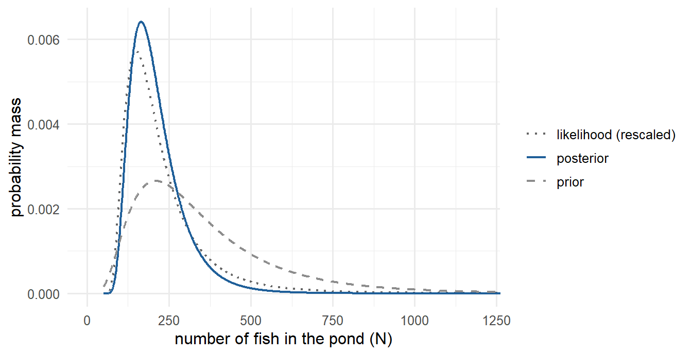
Prior. A local angler says “a few hundred, probably not more than a thousand”. A log-normal distribution with median 300 and log-scale SD 0.6 puts about 95% of its mass between roughly 90 and 1000. Restrict it to $N = 50, \dots, 3000$ and rescale so it sums to one.

Bayes’ rule on a grid. For every candidate $N$: multiply prior × likelihood, then divide by the sum over all $N$.

Figure 1: Prior (dashed), likelihood rescaled to sum to one (dotted) and posterior (solid) for the number of fish.

The posterior sits between the prior (median 300) and the likelihood (peak near 150): posterior mode 165, median 195, mean 213, and a 90% credible interval from 115 to 372. The prior pulls the estimate up because five recaptures out of 25 is little data. The likelihood’s long right tail (large ponds are hard to rule out with few recaptures) is tamed by the prior’s belief that ponds of 2,000 fish are unusual.

Two conditions for this to work, from the notes’ abbreviated workflow:

the likelihood must be defined for every value the prior allows (it may be zero for some), and
at least some values with non-zero prior must give the observed data non-zero probability. If the prior only allowed $N < 50$, no posterior would exist.

Nothing, because the data decide the posterior

It moves to larger N, since the data are weak

It moves to smaller N, towards the likelihood peak

It becomes identical to the new, wider prior

With little data the prior has a large influence. A prior centred on 1,000 pulls the posterior upwards. More recaptures (more data) would make the likelihood narrower and reduce the prior’s influence.

1.5 Summarising a posterior

The posterior is the answer. Summaries are chosen for the reader and the decision at hand.

Summary	Definition	Best under loss…
Posterior mean	$E[\theta \mid y]$	squared error
Posterior median	50th percentile	absolute error
Posterior mode (MAP)	$\arg\max_\theta p(\theta \mid y)$	“all or nothing” (0–1 loss)
Posterior SD	SD of the posterior	describes uncertainty about $\theta$
Equal-tailed 95% credible interval	2.5th to 97.5th percentile	easy, works with transformations
95% highest posterior density (HPD) interval	shortest region containing 95%	can be several pieces if the posterior has several modes

A 95% credible interval means what people usually want a confidence interval to mean: given the model, the prior and the data, $\theta$ lies in the interval with probability 0.95.

Transformations. Because a monotone transformation keeps the order of values, interval endpoints transform directly: if $[-0.40, 0.10]$ is a 95% credible interval for a log relative risk, then $[e^{-0.40}, e^{0.10}] = [0.67, 1.11]$ is a 95% credible interval for the relative risk. Means do not: $E[e^{\theta}] \neq e^{E[\theta]}$. The median transforms directly because it is a percentile.

With a sample of draws (from Module 3 on, MCMC gives you draws from the posterior), every summary becomes an average or a percentile over draws. A derived quantity, such as a ratio of two parameters, is computed draw by draw, which keeps the correlation between parameters intact.

Common confusion: three different spreads

Data SD ($\sigma$): how much individual observations vary. Posterior SD of a mean: how uncertain you are about the mean; it shrinks as $n$ grows, like a standard error. Posterior predictive SD: how uncertain you are about one new observation; it never shrinks below $\sigma$. A larger $\sigma$ usually means larger posterior and predictive SDs too, but they answer different questions.

The posterior mean OR is exactly exp(0.40)

The 95% interval for OR is [exp(0.10), exp(0.70)]

The posterior SD of OR is exp of the SD of log(OR)

Transforming an interval needs the delta method

Percentiles (and so equal-tailed interval endpoints and the median) survive monotone transformations. Means and SDs do not: E[exp(θ)] > exp(E[θ]) for a spread-out posterior. With draws you would simply compute exp() for every draw and summarise the result.

1.6 Posterior predictive distributions

Bayesian models are generative: given parameter values, you can simulate new data. Integrating over the posterior gives the posterior predictive distribution:

\[p(\tilde y \mid y) = \int p(\tilde y \mid \theta)\, p(\theta \mid y)\, d\theta\]

It is easiest to compute by Monte Carlo:

Posterior predictive by Monte Carlo

Repeat many times: (a) draw $\theta^{(s)}$ from the posterior; (b) draw a new $\tilde y^{(s)}$ from $p(y \mid \theta^{(s)})$.
Summarise the $\tilde y^{(s)}$: a mean, a probability such as $P(\tilde y \geq 10)$, or an expected loss.

Fish example: next week you catch 40 fish. Each posterior draw of $N$ gives one simulated number of marked fish. Because $N$ is uncertain, the predictive distribution is wider than a hypergeometric distribution with $N$ fixed at its posterior mean. Plugging in a single best guess underestimates uncertainty.

To check whether you ran enough Monte Carlo draws, rerun the simulation and look at how much the answer changes: that variation is the Monte Carlo error. More draws shrink it at the rate $1/\sqrt{\text{number of draws}}$.

Conditionally generative models. A regression model predicts $y$ given $X$; it does not model the covariates themselves. That is fine when you choose $X$ (a dose, a treatment). Not every method is generative: a permutation test gives a p-value but cannot say what the next observation will look like.

Because Monte Carlo sampling adds noise

It also includes the uncertainty about θ itself

Because the prior is added to the likelihood twice

It is not wider; the two are identical

Predictive uncertainty = sampling variation of a new observation + uncertainty about the parameter. Fixing θ drops the second part.

1.7 The Bayesian workflow, abbreviated

The notes give a four-step version here and expand it in Module 6:

Full probability model for everything: observed data, unknown parameters, future or missing data. Requires knowing the research question and how the data were collected.
Prior: express the available information about the unknowns as a joint prior distribution.
Condition on the data: compute the posterior (and posterior predictive) of the quantities of interest.
Evaluate: does the model fit the data? Are the conclusions reasonable? How sensitive are they to the model and the prior?

Step 4 usually sends you back to step 1 or 2: the workflow is a loop, not a line. Modules 3 and 4 give the tools for step 4.

1.8 Confidence intervals are not credible intervals

Both are abbreviated “CI” and with large samples they often agree numerically. They answer different questions.

95% confidence interval

A property of the procedure: if the experiment were repeated infinitely often, 95% of the intervals produced would contain the true value. Says nothing about this interval.

95% credible interval

A property of this posterior: given the model, prior and data, the parameter lies in the interval with probability 0.95.

Why a confidence interval cannot be read as a credible interval (the notes’ argument, with made-up numbers):

Coverage is about the procedure, not the interval. “Flip a coin: heads, report $(-\infty, \infty)$; tails, report the single point $\{0\}$” is a valid 50% confidence procedure for any non-zero parameter. It never uses the data. Its intervals are either useless or almost certainly wrong, yet the procedure has exact 50% coverage. So the width of a confidence interval does not by itself measure precision.
Several valid procedures give different intervals for the same data. With 4 successes out of 20:

Interval	Lower	Upper
Wald 95% CI	0.025	0.375
Wilson 95% CI	0.081	0.416
Exact (Clopper–Pearson) 95% CI	0.057	0.437
95% credible interval, Beta(1, 1) prior	0.082	0.419

If every valid 95% confidence interval were a 95% probability statement about $\theta$, the region between the Wilson and exact limits would have to contain both 0% and a positive share of the probability. That is a contradiction. So confidence intervals are not automatically probability statements; at most one procedure could coincide with some posterior, and not because it is a confidence procedure.

A credible interval has no such contradiction: one prior + one model + one dataset gives exactly one posterior. Two people with different priors get different posteriors, just as two people with different data or models would.

Do credible intervals have 95% coverage in repeated experiments? Not in general. Coverage depends on how the prior relates to the true value: a prior that puts zero probability on the true value gives zero coverage. Module 2, Section 2.8 shows this in a simulation.

Common confusion: “95% of the time, the true value lies in my confidence interval”

The true value is fixed and your interval is fixed: it either contains the value or not. The 95% refers to the long run of hypothetical repetitions. The sentence “there is a 95% probability that the effect lies between A and B” is a credible-interval statement and needs a prior.

Correct, that is the definition of a confidence interval

That is a credible-interval statement; it needs a prior

Correct, as long as the sample size is above 30

Only true for the exact interval, not for the Wald one

The 95% of a confidence interval refers to the procedure over repeated samples. A probability statement about the parameter itself requires a posterior, and so a prior. With a flat prior and a large sample the numbers are often close, which is why the confusion is common.

1.9 Hypothesis tests and Bayes factors

You can compute $P(\theta > 0 \mid y)$ from a posterior. Two cautions from the notes:

It depends on the prior probability that $\theta > 0$. If you then dichotomise at 0.05, two reasonable priors can give 0.049 and 0.051 and opposite decisions.
For a continuous parameter $P(\theta = 0 \mid y) = 0$: a point null always has zero posterior probability.

The Bayes factor compares whole models instead:

\[\underbrace{\frac{p(m_1 \mid y)}{p(m_2 \mid y)}}_{\text{posterior odds}} = \underbrace{\frac{p(y \mid m_1)}{p(y \mid m_2)}}_{\text{Bayes factor}} \times \underbrace{\frac{p(m_1)}{p(m_2)}}_{\text{prior odds}}\]

BF > 1 favours $m_1$. The Bayes factor does not depend on the prior odds of the models, but it does depend on the priors for the parameters inside each model: a vague prior for an effect in $m_1$ spreads prior mass over huge effects and lowers $p(y \mid m_1)$. You must specify what the alternative hypothesis looks like. The course notes do not use hypothesis testing after Module 1. Later modules compare models by predictive performance instead (Module 4).

When does the Bayesian answer differ most?

Small samples and strong prior information: the prior visibly moves the answer (the fish example).
Unique events and decisions: a probability for this patient, this trial, or an expected loss.
Parameters near a boundary (proportions near 0 or 1, variances near 0), where classical intervals can include impossible values.
With large samples and weak priors the likelihood dominates and Bayesian and classical results usually agree numerically, though their interpretations still differ.

Limitations

The answer depends on the prior and the model. That dependence is visible and can be checked (sensitivity analysis), but it cannot be removed.
Translating vague knowledge (“probably small”) into a specific distribution is hard, and “I have no idea” cannot be expressed exactly (see flat priors in Module 2).
A grid over all parameter values only works for one or two parameters. Beyond that, computation needs MCMC (Module 3).

Part B · Practice in the browser

Interactive R

Cells marked Run Code run R in your browser. The first run on a page takes a few seconds while R loads.

Exercise 1 · Screening. The function computes the positive predictive value.

What is the PPV in a general population where the prevalence is 0.2%?
Which prevalence gives a PPV of 0.5? Try values, or solve with uniroot().
Keep prevalence at 2%. Which matters more for PPV here: raising sensitivity to 0.99 or raising specificity to 0.99?

Model answer

ppv(0.002, 0.95, 0.90) ≈ 0.019. Fewer than 2 in 100 positives have the condition.
uniroot(function(p) ppv(p, 0.95, 0.90) - 0.5, c(0.001, 0.5))$root ≈ 0.095, about 9.5%.
Specificity: ppv(0.02, 0.99, 0.90) ≈ 0.17 but ppv(0.02, 0.95, 0.99) ≈ 0.66. With a rare condition, false positives come from the large healthy group, so specificity dominates.

Exercise 2 · The fish posterior on a grid.

Replace the prior with a flat one (prior <- rep(1, length(pond_size)), then normalise). How do the mean and the 90% interval change? Why does the upper limit depend on the arbitrary cut-off at 3000?
Suppose recaptured had been 15. Rerun with the log-normal prior. Does the prior still matter much?
What is the posterior probability that the pond holds more than 400 fish?

Model answer

The mean rises (about 230) and the 90% interval widens to about 106–477. With a flat prior the long right tail of the likelihood is not tamed; with too few recaptures, very large ponds stay somewhat plausible. Change the grid to 50:10000 and the mean moves again: a “flat” prior on a bounded grid is still a choice.
With 15 recaptures the likelihood is concentrated near 50 fish, and prior and flat-prior posteriors almost agree. More data means less prior influence.
sum(posterior[pond_size > 400]) ≈ 0.035.

Exercise 3 · Posterior predictive by Monte Carlo. Run after Exercise 2 (it uses posterior).

Why is sd_full larger than sd_plugin?
Run the cell three times. How much does prob_10_or_more change? What does that tell you about the Monte Carlo error with 20,000 draws?

Model answer

sd_full includes uncertainty about $N$ as well as the randomness of the catch; the plug-in version pretends $N$ is known.
It changes in the third decimal. That variation is the Monte Carlo error; it is small compared with the uncertainty the probability expresses, so 20,000 draws is enough here.

Why-questions

Why is Bayes’ rule uncontroversial but Bayesian statistics debated?

Bayes’ rule is a theorem of probability. The debate is about whether unknown fixed quantities (parameters, hypotheses, unique events) may have probability distributions, and so whether a prior may be used at all.

Why does the prior matter less as the sample grows?

The likelihood is a product over observations, so it becomes more and more concentrated while the prior stays the same. Eventually the likelihood dominates the product prior × likelihood. The exception: values with zero prior probability stay impossible whatever the data say.

Why should the posterior predictive not use a single best estimate?

A single estimate ignores the uncertainty about the parameter, so predictions are too narrow and rare events look rarer than they are. Tail events (extreme values, rare adverse outcomes) are where this matters most.