Module 3 — Model Fitting with Markov Chain Monte Carlo
The curse of dimensionality · Monte Carlo error · rejection sampling · Gibbs · Metropolis · HMC and NUTS · trace plots, R-hat and ESS · brms · working with draws
Conjugate priors and grids got us exact posteriors for one or two parameters. Real models have dozens or hundreds: a regression with ten covariates, a mixed model with one term per hospital. A grid is hopeless there (1,000 points per parameter and 100 parameters is \(10^{300}\) evaluations), and there is no formula. We need a way to get the posterior without ever computing the normalising integral.
Markov chain Monte Carlo (MCMC) does this. It takes a random walk through parameter space, designed so that the walk spends time in each region in proportion to its posterior probability. After a warm-up, the visited points are (dependent) draws from the posterior, and every summary from Module 1 (means, percentiles, probabilities, predictions) becomes an average over draws. The trick that avoids the integral: the algorithms only ever need ratios of the unnormalised posterior, prior × likelihood, and the unknown constant cancels in a ratio.
The price is that MCMC is only guaranteed to work eventually. In practice you must check that the chains have converged and that you have enough effectively independent draws. Trace plots, R-hat and effective sample size are the tools, and learning to read them is a syllabus outcome.
You will rarely write a sampler yourself. brms translates an R formula into a Stan program and runs the No-U-Turn Sampler (NUTS), a form of Hamiltonian Monte Carlo. This page explains what happens inside, then moves to brms in RStudio.
NoteSources, reading and seminar
Course notes: Module 3 “Model fitting with Markov Chain Monte Carlo” (pp. 97–162). Reading deadline: Seminar 3, Monday 21 September 2026. From this module on, the course uses brms, which needs RStan and a C++ toolchain (Rtools on Windows).
Optional: McElreath, Statistical Rethinking, chapter 9 (MCMC) and chapters 4–5 (linear models). The notes recommend Chi Feng’s interactive MCMC demos (https://chi-feng.github.io/mcmc-demo/): try the Metropolis algorithm on the “banana” and “donut” targets and then NUTS.
Examples on this page (Gamma posterior, runners’ heart rate, a blood pressure trial, weight recorded twice) are written for this app.
TipBefore you start: three things you need
Monte Carlo = estimate by simulation. If \(\theta^{(1)}, \dots, \theta^{(S)}\) are draws from \(p(\theta \mid y)\), then \(E[g(\theta) \mid y] \approx \frac{1}{S}\sum_s g(\theta^{(s)})\) for any function \(g\). With independent draws the error shrinks like \(1/\sqrt{S}\).
Standard error of a mean. \(\text{SD}/\sqrt{n}\) for independent observations. With positively correlated observations the true standard error is larger: correlated draws carry less information.
Unnormalised posterior. \(q(\theta) = p(y \mid \theta)\,p(\theta)\) is proportional to the posterior. The ratio \(q(\theta_a)/q(\theta_b)\) equals the ratio of posterior densities: the normalising constant cancels.
Part A · Concepts
3.1 The curse of dimensionality
- Summaries are not enough. The mean and SD do not determine a distribution: a Student-t and a normal with the same mean and SD have different 95th percentiles. We want the whole posterior, including skewness and tails.
- Grids grow exponentially. If one parameter needs 1,000 grid points, \(p\) parameters need \(1000^p\). Even a smarter rule with 2 points per parameter needs \(2^{195} \approx 5 \times 10^{58}\) evaluations for a model with one dummy per country.
- Monte Carlo breaks the curse: its error depends on the number of (effective) draws, not directly on the number of parameters.
3.2 Monte Carlo and its standard error
Monte Carlo methods use random numbers but converge to fixed answers. The price is Monte Carlo error: rerun and you get a slightly different number.
- Estimate it by rerunning and taking the SD of the results, or (for independent draws) by \(\text{SD}/\sqrt{S}\).
- It shrinks like \(1/\sqrt{S}\): 16 times more draws for 4 times less error.
- Keep it small relative to the posterior uncertainty. The notes’ rule: the Monte Carlo standard error (MCSE) of a posterior mean should be at least 10 times smaller than the posterior SD, preferably 100 times.
The bootstrap is a familiar Monte Carlo method (resample, refit, take the SD of the estimates). It has its own Monte Carlo error, usually ignored because 1,000+ replicates make it small. Bootstrap replicates are independent; MCMC draws are not (Section 3.10).
3.3 Rejection sampling
To sample from a target \(f\) when you can sample from a proposal \(g\) and know \(c = \max f(x)/g(x)\):
- Draw \(x \sim g\) and \(u \sim \text{Uniform}(0, 1)\).
- Accept \(x\) if \(u \leq f(x) / (c\, g(x))\); otherwise discard it.
Accepted draws are exact, independent draws from \(f\). The acceptance rate is \(1/c\), and \(c\) grows exponentially with the number of dimensions when \(g\) does not match \(f\). Rejection sampling is fine in one dimension and hopeless in fifty. MCMC fixes this by proposing locally, near the current point.
3.4 Markov chains: the generic recipe
A (first-order) Markov chain generates each new value from the current one only: \(\theta^{(t)} \sim T(\theta \mid \theta^{(t-1)})\). MCMC algorithms choose the transition distribution \(T\) so that the chain’s long-run distribution is the posterior:
- Start at some \(\theta^{(0)}\).
- Draw \(\theta^{(t)}\) from \(T(\cdot \mid \theta^{(t-1)})\).
- Repeat. After a warm-up of \(b\) iterations, treat \(\theta^{(b+1)}, \dots, \theta^{(q)}\) as draws from \(p(\theta \mid y)\).
The Markov property is a cost, not a feature: consecutive draws are autocorrelated, so 4,000 draws carry less information than 4,000 independent ones (Section 3.10). Regions with high posterior density are visited often and low-density regions rarely, but the chain can visit anywhere with non-zero density.
3.5 The Gibbs sampler
If you can sample from each full conditional \(p(\theta_j \mid \theta_{-j}, y)\), update one parameter (or block) at a time:
\[\theta_1^{(t)} \sim p(\theta_1 \mid \theta_2^{(t-1)}, \dots, y), \quad \theta_2^{(t)} \sim p(\theta_2 \mid \theta_1^{(t)}, \theta_3^{(t-1)}, \dots, y), \quad \dots\]
- Needs the conditionals in closed form, in practice conjugate priors for each parameter. This is why older software (BUGS, JAGS) encourages conjugate priors.
- Moves parallel to the axes, so it is very slow when parameters are strongly correlated: each conditional is narrow and the chain creeps along a diagonal ridge.
- Natural for hierarchical models, where the conditionals are simple. Multiple imputation by chained equations is essentially a Gibbs sampler.
3.6 Metropolis and Metropolis–Hastings
Metropolis algorithm
- Start at \(\theta^{(0)}\).
- Propose \(\theta^* \sim J(\theta^* \mid \theta^{(t-1)})\) from a symmetric jumping distribution, e.g. \(N(\theta^{(t-1)}, \text{step}^2)\).
- Compute \(r = \dfrac{p(\theta^* \mid y)}{p(\theta^{(t-1)} \mid y)} = \dfrac{p(y \mid \theta^*)\,p(\theta^*)}{p(y \mid \theta^{(t-1)})\,p(\theta^{(t-1)})}\). The normalising constant cancels.
- Draw \(u \sim \text{Uniform}(0,1)\). If \(u \leq r\), accept: \(\theta^{(t)} = \theta^*\). Otherwise stay: \(\theta^{(t)} = \theta^{(t-1)}\), and the old value is counted again.
- Uphill moves (\(r \geq 1\)) are always accepted; downhill moves are accepted with probability \(r\). That is what makes the chain explore the whole posterior rather than climb to the mode (always accepting uphill and never downhill would be hill climbing, an optimiser).
- Tuning. Tiny steps: almost everything is accepted but the chain crawls. Huge steps: almost everything is rejected and the chain sits still. An acceptance rate of roughly 0.2–0.5 works best (try it in Part B).
- Metropolis–Hastings allows asymmetric proposals by using \(r = \dfrac{p(\theta^* \mid y)/J(\theta^* \mid \theta^{(t-1)})}{p(\theta^{(t-1)} \mid y)/J(\theta^{(t-1)} \mid \theta^*)}\). Plain Metropolis is the special case \(J\) symmetric.
The chain has converged and mixes very well
The steps are too small, so exploration is slow
The posterior is flat, so every move is uphill
The proposal is too wide for this posterior
Tiny proposals land where the density is almost the same, so r ≈ 1 and nearly all are accepted, but each step moves very little. The draws are highly autocorrelated and the effective sample size is low. A very low acceptance rate signals the opposite problem (steps too large).
3.7 Hamiltonian Monte Carlo and NUTS
Random-walk proposals are local and blind to the shape of the posterior. Hamiltonian Monte Carlo (HMC) uses the gradient of the log posterior to make long, well-aimed proposals:
- Picture the negative log posterior as a landscape and a frictionless marble on it. Give the marble a random push (momentum) and follow its path for a while with the leapfrog integrator. Where it stops is the proposal. It speeds up downhill and slows uphill, so it follows the shape of the posterior.
- A Metropolis-style accept/reject step corrects for errors in the path. Proposals far away can still be accepted with high probability; Stan targets an acceptance rate of 0.8.
- NUTS (No-U-Turn Sampler) chooses the path length automatically: it stops when the trajectory starts to turn back on itself. It is Stan’s default.
- Warm-up in Stan both discards early draws and tunes the step size and metric. Warm-up draws are never used for inference.
What can go wrong, and what brms tells you:
| Warning | Meaning | Typical fix |
|---|---|---|
| Divergent transitions | The leapfrog path broke down in a region of sharp curvature (often a funnel in a hierarchical model). Draws may be biased. | Increase adapt_delta (e.g. 0.95, 0.99) for smaller steps; better, reparameterise or use more informative priors |
| Maximum treedepth exceeded | Paths hit the length limit, often because the posterior is very flat or elongated in some direction | Look for poorly identified parameters (Section 3.13); max_treedepth only helps with efficiency |
| High R-hat, low ESS | Chains disagree or are too autocorrelated | See Sections 3.8–3.10 |
HMC needs continuous parameters (the marble needs a smooth surface), so Stan cannot sample discrete parameters directly.
3.8 Convergence I: trace plots
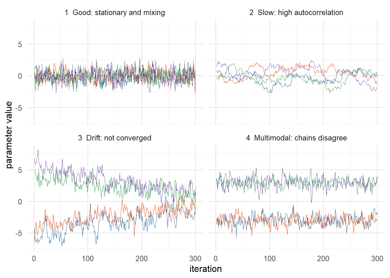
Run several chains (brms default: 4) from different starting points. If they have all converged to the posterior they should be indistinguishable. A trace plot shows each parameter’s value against iteration, one colour per chain. Ask:
- Are the chains stationary (no trend)?
- Do they mix (overlap, cross each other constantly)?
- Do they have the same mean and spread?
| Pattern | Likely cause | What to do |
|---|---|---|
| Autocorrelated but overlapping (2) | Slow exploration | Run longer; check ESS; reparameterise if extreme |
| Drift (3) | Warm-up too short; very slow chain | Run much longer; simplify or reparameterise |
| Chains in different places (4) | Multimodal posterior; poor identification | Rethink model and prior; running longer rarely rescues this |
A single chain split in two can look fine while stuck in one mode: several chains from dispersed starting values are more likely to reveal a second mode. No diagnostic proves convergence: they can only detect non-convergence.
3.9 Convergence II: R-hat
The Gelman–Rubin statistic compares between-chain and within-chain variance, like an ANOVA. With \(m\) chains of length \(q\):
\[W = \frac{1}{m}\sum_j s_j^2, \qquad B = \frac{q}{m-1}\sum_j (\bar\theta_{\cdot j} - \bar\theta_{\cdot\cdot})^2, \qquad \widehat{\text{var}}^+ = \frac{q-1}{q}W + \frac{1}{q}B, \qquad \hat R = \sqrt{\frac{\widehat{\text{var}}^+}{W}}.\]
- If all chains sample the same distribution, \(B\) is small and \(\hat R \approx 1\).
- Chains stuck apart, or still travelling from their starting values, inflate \(B\) and give \(\hat R > 1\).
- Modern R-hat (the one brms reports) splits each chain in half first, so a single drifting chain is also detected, and uses rank-normalisation so heavy tails do not break it.
Rules of thumb. The course notes use \(\hat R < 1.1\). brms warns above 1.05. Current Stan advice (Vehtari et al., 2021) is \(\hat R < 1.01\) for final results. Check R-hat for every parameter; look at trace plots for the ones that fail.
About 1.00, since each chain looks stable
Well above 1, as the chain means differ
Exactly 1.1, the conventional cut-off value
Undefined, since the means cancel out
B is large relative to W, so var⁺ is much larger than W and R-hat is far above 1. This is the multimodal pattern in panel 4: each chain looks fine on its own, but they disagree.
3.10 Convergence III: effective sample size and MCSE
With autocorrelation \(\rho_t\) at lag \(t\), \(m\) chains of \(q\) draws carry as much information as
\[n_\text{eff} = \frac{mq}{1 + 2\sum_{t=1}^{\infty} \rho_t}\]
independent draws. Strong autocorrelation means a small ESS. The MCSE of the posterior mean is about \(\text{posterior SD}/\sqrt{n_\text{eff}}\).
brms reports two ESS values:
- Bulk_ESS: for the centre of the distribution (mean, median, SD).
- Tail_ESS: for the 5% and 95% quantiles, and so for credible interval limits. Tails need more draws.
Rules of thumb (course notes). Bulk ESS ≥ 1,000 for posterior means and SDs: then \(1/\sqrt{1000} \approx 3\%\), so the MCSE is about 3% of the posterior SD. Stan’s warnings trigger below 100 per chain. For extreme quantiles or rare events you need more.
Thinning (keeping every \(k\)-th draw) lowers autocorrelation but throws information away. With NUTS the advice is to keep all post-warm-up draws; thinning only helps when memory is the bottleneck.
Nothing, since R-hat shows convergence
Run more iterations to raise the ESS
Thin the chains to reduce autocorrelation
Increase adapt_delta to 0.99 and refit
R-hat ≈ 1 says the chains agree; ESS says how precise the Monte Carlo estimates are. With ESS = 150 the MCSE is about 8% of the posterior SD. Running longer raises the ESS. Thinning would lower it further.
3.11 Fitting models with brms
fit <- brm(
  y ~ x1 + x2,                    # R formula, like lm()/glm()
  family = gaussian(),            # the likelihood (bernoulli, binomial, poisson, student, ...)
  prior = c(
    prior(normal(0, 5), class = "Intercept"),
    prior(normal(0, 1), class = "b"),          # all slopes; or coef = "x1" for one
    prior(exponential(1), class = "sigma")
  ),
  data = d,
  chains = 4, iter = 2000,        # half of iter is warm-up: 4 x 1000 = 4000 draws kept
  seed = 123                      # brms ignores set.seed(); use seed =
)- The first call compiles a C++ program: a minute or more. Sampling is often faster than compiling. Use
file = "name"to save the fit and skip refitting next time. get_prior(y ~ x1 + x2, data = d)lists every parameter that needs a prior, with brms defaults. Defaults are not “no prior”: slopes get flat priors, the intercept andsigmaget Student-t priors scaled to the data.options(mc.cores = 4)runs the chains in parallel.
Reading summary(fit). Check diagnostics first, estimates second.
| Column | Meaning |
|---|---|
Estimate, Est.Error |
posterior mean and posterior SD |
l-95% CI, u-95% CI |
2.5% and 97.5% posterior quantiles (a credible interval, despite the name) |
Rhat, Bulk_ESS, Tail_ESS |
convergence diagnostics (Sections 3.9–3.10) |
In as_draws_df(fit) the parameters are called b_Intercept, b_x1, sigma, …; lprior and lp__ are the log prior and log posterior (unnormalised), used internally. brms centres predictors internally, so Intercept (the centred intercept) and b_Intercept can differ when predictors are not centred.
3.12 Working with draws: linpred, epred and predict
The syllabus asks you to “prepare tables and figures that summarise the estimand(s) … by manipulating the sample from the joint posterior”. Three brms functions, each returning a matrix of draws × observations:
| Function | Gives draws of… | Example (logistic model) |
|---|---|---|
posterior_linpred(fit) |
the linear predictor \(\eta_i = \alpha + \beta x_i\) | log-odds |
posterior_linpred(fit, transform = TRUE) or posterior_epred(fit) |
the expected outcome \(E[\tilde y_i] = g^{-1}(\eta_i)\) | probability (epred × trials for binomial) |
posterior_predict(fit) |
a new observation \(\tilde y_i\) | 0 or 1 |
Add newdata = for new covariate values. predict is always wider than epred: it adds the outcome’s own randomness to the uncertainty about the mean.
Any estimand, computed draw by draw. Take as_draws_df(fit), compute your quantity for each row, then summarise:
draws <- as_draws_df(fit)
draws$std_effect <- draws$b_treated / draws$sigma          # standardised effect
quantile(draws$std_effect, c(0.025, 0.5, 0.975))
mean(draws$b_treated < -5)                                 # P(effect < -5 | y)
Computing from rows of the same draw keeps the posterior correlation between parameters. Mixing values from different draws (for example, the mean of one parameter with a quantile of another) does not.
3.13 Poorly identified models
If the data cannot distinguish some parameter combinations, the posterior is a long flat ridge: only a combination is identified. Example: body weight entered twice, once in kg and once in pounds. Only \(\beta_\text{kg} + 2.2046\,\beta_\text{lb}\) is identified. With vague priors the chains wander along the ridge: huge R-hat, tiny ESS, maximum-treedepth warnings (Task 3.3 below).
- A more informative prior makes the posterior proper and the chains converge, but then the split between the two coefficients comes entirely from the prior.
- The honest fix is usually a simpler model. Poor convergence is often the first sign of a model problem: nearly collinear predictors, many interactions with sparse cells, too many latent variables.
The notes’ advice: when chains misbehave, fit a simpler model to see whether identifiability is the cause.
When to use MCMC (and brms)
- Any model without a conjugate solution: GLMs, mixed models, robust (Student-t) likelihoods, non-standard priors.
- When you want the joint posterior for derived quantities (ratios, contrasts, rankings, predictions) with correct uncertainty.
- brms covers most regression models you will meet (GLMM, GAMM, ordinal, survival, multivariate) with lme4-like syntax.
Limitations
- Only asymptotic guarantees. Diagnostics detect non-convergence; they cannot prove convergence.
- Slow for big models or big data; compilation adds minutes.
- HMC cannot handle discrete parameters directly.
- Convergence says nothing about whether the model is right: a wrong model can converge perfectly (Module 4).
Part B · Practice
In the browser: a Metropolis sampler you can tune
NoteInteractive R
Runs in your browser. The target is the Gamma(7, 3.5) posterior from Module 2, Section 2.10, so you can compare MCMC with the exact answer.
- Which step size gives a chain you would trust? Describe what goes wrong in the other two.
- With
step = 1, discard the first 500 draws and compare the mean and 95% interval with the exact Gamma(7, 3.5): mean 2.0, interval 0.80–3.73.
TipModel answer
- Step 1 (acceptance about 0.6) moves quickly and mixes. Step 0.05 accepts 98% of proposals but crawls: it needs about 500 iterations just to walk down from 6, and the trace is a slow wave. Step 15 accepts only about 6%: long flat stretches where the chain stands still.
run <- metropolis(20000, 1, 6); keep <- run$draws[-(1:500)]; c(mean(keep), quantile(keep, c(.025, .975)))gives about 2.0 and 0.8–3.7, matching the exact answer up to Monte Carlo error.
- Change the step size to 0.05 in the
sapplyline. What happens to R-hat and the ESS? - Why is the ESS smaller than the number of draws even for a well-tuned chain?
TipModel answer
- With step 1 we got R-hat ≈ 1.00 and an ESS of about 300 from 2,000 draws. With step 0.05 the chains move so slowly that they still disagree after warm-up: R-hat ≈ 1.2–1.3 and the ESS collapses to about 10.
- Consecutive Metropolis draws are positively correlated (a rejected proposal repeats the previous value exactly). Correlated draws carry less information than independent ones.
In RStudio: brms tasks
ImportantHow the RStudio tasks work
Each task simulates its own data, so you can run it straight away. Try it yourself first, then open the solution. The solutions were run with brms 2.23; your numbers will differ slightly (Monte Carlo error). Download all Module 3 tasks as one script: module3-tasks.R.
Task 3.1 · Your first brms model: an intercept and a standard deviation
Twelve runners’ resting heart rates (simulated): set.seed(510); runners <- data.frame(heart_rate = round(rnorm(12, mean = 58, sd = 7))).
Fit heart_rate ~ 1 with a Gaussian likelihood, prior normal(70, 15) for the intercept and exponential(0.1) for sigma.
- Check the diagnostics before anything else. Are R-hat and ESS acceptable?
- Compare the posterior mean with the sample mean. Which way did the prior pull, and why so little?
- Compute \(P(\mu < 60 \mid y)\) and a 90% credible interval from the draws.
TipSolution
fit_hr <- brm(heart_rate ~ 1, family = gaussian(),
              prior = c(prior(normal(70, 15), class = "Intercept"),
                        prior(exponential(0.1), class = "sigma")),
              data = runners, chains = 4, iter = 2000, seed = 510, refresh = 0)
summary(fit_hr)
plot(fit_hr)
draws_hr <- as_draws_df(fit_hr)
mean(draws_hr$b_Intercept < 60)
quantile(draws_hr$b_Intercept, c(0.05, 0.95))
What we got: Intercept 58.56 (SD 2.55), sigma 8.92, Rhat 1.00, Bulk_ESS ≈ 2,400 for both. Diagnostics fine. The sample mean is 58.25, so the prior (centred on 70) pulled the estimate up by only 0.3: the prior SD of 15 is wide compared with the data’s standard error (about 9/√12 ≈ 2.6). \(P(\mu < 60) \approx 0.73\); 90% interval 54.4 to 62.8.
Task 3.2 · A treatment effect, and quantities computed from draws
Simulated trial, 30 patients per arm:
set.seed(511)
trial <- data.frame(treated = rep(c(0, 1), each = 30))
trial$sbp_change <- rnorm(60, mean = -2 - 6 * trial$treated, sd = 8)
Fit sbp_change ~ treated with priors normal(0, 20) (Intercept), normal(0, 10) (b) and exponential(0.1) (sigma).
- Compute the posterior of the standardised effect \(\beta/\sigma\) and a 95% interval.
- What is the probability that the drug lowers SBP by more than 5 mmHg?
- Use
posterior_linpred()andposterior_predict()withnewdata = data.frame(treated = c(0, 1)). Compare their SDs and explain the difference. - Rebuild both for the treated group by hand from
as_draws_df()and check that you get the same.
TipSolution
fit_trial <- brm(sbp_change ~ treated, family = gaussian(),
                 prior = c(prior(normal(0, 20), class = "Intercept"),
                           prior(normal(0, 10), class = "b"),
                           prior(exponential(0.1), class = "sigma")),
                 data = trial, chains = 4, iter = 2000, seed = 511, refresh = 0)
draws_trial <- as_draws_df(fit_trial)
draws_trial$std_effect <- draws_trial$b_treated / draws_trial$sigma
quantile(draws_trial$std_effect, c(0.025, 0.5, 0.975))
mean(draws_trial$b_treated < -5)

new_patients <- data.frame(treated = c(0, 1))
apply(posterior_linpred(fit_trial, newdata = new_patients), 2, sd)
apply(posterior_predict(fit_trial, newdata = new_patients), 2, sd)

mu_treated <- draws_trial$b_Intercept + draws_trial$b_treated
y_treated  <- rnorm(nrow(draws_trial), mu_treated, draws_trial$sigma)
c(sd(mu_treated), sd(y_treated))
What we got: treated −5.89 (95% CrI −9.39 to −2.26), sigma 7.24. Standardised effect: median −0.82, 95% interval −1.35 to −0.30. \(P(\beta < -5) \approx 0.69\).
SD of the mean (linpred) ≈ 1.3 in each arm; SD of a new patient (predict) ≈ 7.4. The mean is estimated from 30 patients, but one new patient also varies with SD σ ≈ 7.2 around that mean: \(\sqrt{1.3^2 + 7.2^2} \approx 7.4\). The by-hand versions give the same (1.29 and 7.45).
Task 3.3 · When the chains do not converge
The same body weight in two units:
set.seed(512)
bodyweight <- data.frame(weight_kg = rnorm(50, mean = 75, sd = 12))
bodyweight$weight_lb <- bodyweight$weight_kg * 2.2046
bodyweight$sbp <- rnorm(50, mean = 100 + 0.4 * bodyweight$weight_kg, sd = 8)- Fit
sbp ~ weight_kg + weight_lbwith a vaguenormal(0, 1000)prior on the slopes (Interceptnormal(120, 30), sigmaexponential(0.1),iter = 1000). Read the warnings, R-hat and ESS. Look at the trace plots of the two slopes. - Compute
b_weight_kg + 2.2046 * b_weight_lbdraw by draw. Is that well estimated? - Refit with a
normal(0, 1)prior on the slopes. What changes, and what does the prior now decide?
TipSolution
fit_both_vague <- brm(sbp ~ weight_kg + weight_lb, family = gaussian(),
                      prior = c(prior(normal(120, 30), class = "Intercept"),
                                prior(normal(0, 1000), class = "b"),
                                prior(exponential(0.1), class = "sigma")),
                      data = bodyweight, chains = 4, iter = 1000, seed = 512, refresh = 0)
summary(fit_both_vague)
plot(fit_both_vague, variable = c("b_weight_kg", "b_weight_lb"))
draws_vague <- as_draws_df(fit_both_vague)
effect_per_kg <- draws_vague$b_weight_kg + 2.2046 * draws_vague$b_weight_lb
summarise_draws(data.frame(effect_per_kg), "mean", "sd", "rhat", "ess_bulk")
What we got with the vague prior: weight_kg 333 ± 789 and weight_lb −151 ± 358, Rhat 2.68, Bulk_ESS 5, and warnings that 1,843 of 2,000 transitions exceeded the maximum treedepth. The chains wander along the ridge. Yet the identified combination is fine: effect per kg 0.22 (SD 0.11), Rhat 1.00, ESS ≈ 2,000.
With normal(0, 1): the model converges (Rhat ≤ 1.01, ESS ≈ 750), weight_kg 0.02 ± 0.93 and weight_lb 0.09 ± 0.42. The combination is still 0.02 + 2.2046 × 0.09 ≈ 0.22, but how it is split between the two coefficients is decided entirely by the prior. The real fix is to drop one of the two variables.
(The simulation used 0.4 mmHg per kg; with 50 people the estimate 0.22 ± 0.11 is within about two posterior SDs of that.)
Why-questions
NoteWhy does Metropolis only need the unnormalised posterior?
It only uses the ratio \(p(\theta^* \mid y)/p(\theta \mid y)\). The normalising constant appears in both numerator and denominator and cancels. Computing that constant is exactly the integral we could not do.
NoteWhy run several chains rather than one long chain?
Chains started in different places that end up agreeing are evidence of convergence. A single chain stuck in one mode can look perfectly stationary. R-hat needs several chains, and they run in parallel on several cores.
NoteWhy is R-hat ≈ 1 not enough?
R-hat checks that chains agree, not that you have enough information. Also check the ESS (precision of the estimates), divergent transitions (possible bias) and, separately, whether the model fits the data (Module 4).
Spaced review: Modules 1–2
Note1. The Beta(13.8, 9.2) prior is worth how many observations?
a + b − 2 = 21 (notes’ convention). (2.7)