Module 5 — Hierarchical Models and Shrinkage

Complete, no and partial pooling · hyperpriors · shrinkage by group size · reading brms output · new groups · nested and crossed structures · varying slopes · bias–variance · meta-analysis · ranks

Many datasets consist of groups: patients in hospitals, respondents in regions, repeated measurements in patients, studies in a meta-analysis. You then need a parameter per group, and the number of parameters grows with the data. What prior should 200 hospital-specific parameters get? Using the same prior for all of them already says they are similar. A hierarchical model makes that similarity explicit and learns from the data how similar they are.

The model has two levels. Each group’s parameter is drawn from a common population distribution, say $N(\mu, \tau^2)$, and $\mu$ and $\tau$ get priors of their own (hyperpriors). This is the “chicken and egg” of the notes: the group estimates need the population distribution as their prior, and the population distribution is estimated from the groups. The hierarchical model estimates both at once.

The result is partial pooling: each group’s estimate is a compromise between its own data and the population mean, exactly the shrinkage of Module 2. Groups with little data are pulled strongly towards the mean; groups with a lot of data mostly keep their own estimate. Complete pooling (all groups identical) and no pooling (groups unrelated) are the two extremes, reached when $\tau \to 0$ or $\tau \to \infty$.

This is a generalised linear mixed model (GLMM), the model class of your individual project. In brms it is one extra term in the formula: (1 | hospital).

Sources, reading and seminar

Course notes: Module 5 “Hierarchical models and shrinkage” (pp. 217–262). Reading deadline: Seminar 5 (GLMM), October 2026; check TimeEdit for the date. There is also a lecture on hierarchical models.

Optional: McElreath, Statistical Rethinking, chapters 13–14 (multilevel models, varying slopes). Gelman and Hill (2007), Data Analysis Using Regression and Multilevel/Hierarchical Models. The Stan team’s pooling case study: https://mc-stan.org/rstanarm/articles/pooling.html.

Examples on this page (a nurse-led blood pressure programme in 10 clinics, HbA1c targets in 15 primary care clinics, blood pressure over five visits) are written for this app. The notes use infant surgery mortality and a magnesium meta-analysis.

Before you start: three things you need

Shrinkage (2.3). With a normal prior, the posterior mean is $\bar y$ pulled towards the prior mean by the fraction $\frac{\text{SE}^2}{\text{SE}^2 + \sigma_0^2}$. Noisy data → more pull.

Random intercepts (STA240). In lme4, y ~ x + (1 | cluster) gives each cluster its own intercept drawn from $N(0, \sigma_u^2)$. The ICC is $\sigma_u^2 / (\sigma_u^2 + \sigma^2)$. brms uses the same formula syntax.

The logit scale. For binary data the model is linear on the log-odds scale; plogis() converts back to probabilities. A difference of 0.5 on the log-odds scale is an odds ratio of $e^{0.5} \approx 1.65$.

Part A · Concepts

5.1 Why hierarchical models?

The number of parameters grows with the data. One term per child, hospital or study. Flat priors for each give noisy, unstable estimates (and infinite ones for a group where everyone had the outcome).
Similar-yet-distinct groups. Hospitals are not identical (complete pooling is wrong) but not unrelated either (no pooling throws away information).
Something is better than nothing. From Module 1: a good prior plus one observation beats a flat prior plus one observation. For a small group, the other groups provide that prior.
Prediction for new groups needs a distribution of group effects; a model with a separate fixed parameter per group has no such distribution.

5.2 Complete, no and partial pooling

For binomial data from hospitals $j = 1, \dots, J$ ($y_j$ events out of $n_j$):

	Complete pooling	No pooling	Partial pooling
Model	$\text{logit}(p_j) = \alpha$	$\text{logit}(p_j) = \alpha_j$	$\text{logit}(p_j) = \alpha + u_j$
Priors	$\alpha \sim N(\cdot)$	$\alpha_j \sim N(\cdot)$, independently	$u_j \sim N(0, \tau^2)$, $\alpha \sim N(\cdot)$, $\tau \sim$ hyperprior
brms	`y \\| trials(n) ~ 1`	`y \\| trials(n) ~ 0 + hospital`	`y \\| trials(n) ~ 1 + (1 \\| hospital)`
Assumes	all hospitals identical	hospitals unrelated	hospitals similar, how similar is estimated
Hospital estimates	all equal	each from its own data only	own data shrunk towards the mean
Predicts a new hospital?	yes (trivially)	no	yes

0 + hospital gives one parameter per hospital directly (rather than a reference hospital plus differences), so each can get the same prior.

In the partial pooling model, the population-level (“fixed”) effect $\alpha$ is the log-odds in the average hospital; group-level (“random”) effects $u_j$ are deviations from it; $\tau$ is the between-hospital SD. The notes prefer to avoid “fixed” and “random”: in the Bayesian view everything unknown has a distribution.

Figure 1: Estimated share at target in 15 simulated clinics under no pooling (open circles) and partial pooling (filled). The dashed line is the complete-pooling estimate. Arrows show shrinkage; small clinics (left) move most.

Each hospital keeps its own raw estimate

The model is close to complete pooling

The model cannot be fitted with MCMC

The hospitals differ more than the data suggest

τ → 0 means all hospitals share (almost) the same true value, so every estimate is pulled almost fully to the common mean: complete pooling. τ → ∞ gives no pooling.

5.3 The hyperprior

The prior on $\tau$ decides how much pooling the model does a priori; the data update it. Choosing it is harder than choosing a prior for a mean, because intuition about SDs of log-odds is weak.

Common choices: exponential(1) (mean 1), half-normal normal(0, 1) (brms truncates it at 0 for class sd), half Student-t student_t(3, 0, 2.5) (the brms default).
Think on the scale of the linear predictor. On the log-odds scale, $\tau = 1$ means that hospitals one SD apart differ by an odds ratio of $e^{1} \approx 2.7$, and the middle 95% of hospitals span an odds-ratio range of $e^{4} \approx 55$. That is a lot of variation; $\tau$ around 0.2–0.5 is more typical.
With few groups the hyperprior matters. Five or six groups carry little information about $\tau$ (you estimate an SD from five numbers). With 50 groups the data dominate. Task 5.5 shows this.
A flat prior on $\tau$ is possible (the notes do it in the meta-analysis) but can give improper posteriors or divergences; brms may need adapt_delta near 1.

Empirical Bayes estimates $\tau$ first and then plugs it in as if known. The notes’ comparison: it “purchases a duck and hopes for chicken eggs”. It uses the data twice and ignores the uncertainty in $\tau$, so intervals are too narrow.

5.4 How much shrinkage?

For a normal hierarchical model with known group standard errors $s_j$ (the building block of meta-analysis):

\[\hat\theta_j = \frac{\bar y_j / s_j^2 + \mu / \tau^2}{1/s_j^2 + 1/\tau^2} = \bar y_j - \underbrace{\frac{s_j^2}{s_j^2 + \tau^2}}_{\text{shrinkage factor } B_j}\,(\bar y_j - \mu).\]

The shrinkage factor $B_j$ is large when the group’s own estimate is noisy ($s_j$ large: few observations) or the groups are similar ($\tau$ small). This is the Module 2 formula, with the population distribution playing the role of the prior.

Consequences:

Extreme raw estimates usually come from small groups (noise), and they move most. Ranking hospitals on raw rates rewards and punishes small hospitals by chance.
Differences between groups shrink, so credible intervals for differences more often include zero. Gelman, Hill and Yajima (2012) proposed partial pooling as an alternative to multiple-comparison corrections.
Group estimates are biased towards the mean but have lower total error: see 5.9.

5.5 Reading brms output for a hierarchical model

 Family: binomial
Formula: at_target | trials(n_patients) ~ 1 + (1 | clinic)
Multilevel Hyperparameters:
~clinic (Number of levels: 15)
              Estimate Est.Error l-95% CI u-95% CI Rhat Bulk_ESS Tail_ESS
sd(Intercept)     0.76      0.19     0.46     1.22 1.00      956     1673
Regression Coefficients:
          Estimate Est.Error l-95% CI u-95% CI Rhat Bulk_ESS Tail_ESS
Intercept     0.35      0.22    -0.08     0.80 1.00      650     1050

(Output from Task 5.1 below.) “Multilevel Hyperparameters” is the group level: τ. “Regression Coefficients” is the population level. In the draws (as_draws_df(fit)):

Name	Meaning
`b_Intercept`	population-level intercept: log-odds in the average clinic
`sd_clinic__Intercept`	$\tau$: between-clinic SD on the log-odds scale
`r_clinic[C,Intercept]`	$u_C$: clinic C’s deviation from the average (the `r_` prefix = group-level term)
`cor_patient__Intercept__month`	correlation between varying intercepts and slopes (Section 5.8)

Clinic C’s own log-odds is b_Intercept + r_clinic[C,Intercept], computed draw by draw. posterior_linpred(fit) or posterior_epred(fit) does this for you. ranef(fit) summarises the $u_j$; coef(fit) summarises $\alpha + u_j$.

Three different “averages” with a non-linear link: the probability in the average clinic (plogis(b_Intercept)), the average probability over clinics (average plogis(b_Intercept + u) over the distribution of $u$), and the average over patients (weighted by clinic size). They differ. Decide which one your question needs and compute it from the draws.

plogis(mean(b_Intercept)) + mean(r_clinic[D,Intercept])

Per draw: plogis(b_Intercept + r_clinic[D,Intercept])

Per draw: plogis(r_clinic[D,Intercept]) alone

mean(b_Intercept) + mean(sd_clinic__Intercept)

Add the population intercept and the clinic’s deviation within each draw, transform, then summarise. Averaging first and transforming later ignores the non-linearity and the correlation between the two parameters.

5.6 Predictions for existing and new groups

Question	Uses	brms
Clinic D, which is in the data	$\alpha + u_D$	`posterior_epred(fit, newdata = data.frame(clinic = "D", ...))`
The average clinic ($u = 0$)	$\alpha$	`re_formula = NA`
A new clinic	$\alpha + u_\text{new}$, $u_\text{new} \sim N(0, \tau^2)$ drawn per draw	`allow_new_levels = TRUE, sample_new_levels = "gaussian"`

A new clinic’s prediction is wider than any existing clinic’s: you know nothing specific about it, and $\tau$ is itself uncertain. Plugging in posterior means of $\mu$ and $\tau$ and then simulating ignores that uncertainty and is too narrow (the notes’ Exercise 5.1 makes the same point).

A new clinic’s predictive distribution is also the prior for its effect if it later sends data, so the hierarchical posterior provides priors for future groups.

5.7 Nested, crossed and the formula syntax

brms formula	Model	Structure
`y ~ 1 + (1 \\| district)`	$y_i \sim N(\alpha + u_{j[i]}, \sigma^2)$, $u_j \sim N(0, \tau_d^2)$	one grouping factor
`y ~ 1 + (1 \\| state/district)`	$+\; v_{k[j]} + u_{j[i]}$	districts nested in states; same as `(1 \\| state) + (1 \\| state:district)`
`y ~ size + public + (1 \\| district)`	covariates + random intercept	GLMM with predictors
`y ~ size + (1 + size \\| district)`	intercepts and slopes vary, correlated	varying slopes (5.8)
`y ~ size + (0 + size \\| district)`	only slopes vary
`y ~ x + (1 \\| patient) + (1 \\| rater)`	crossed: each patient seen by several raters	not nested
`y ~ x + (1 \\| region) + (1 \\| round)`	crossed: region × survey round	the project starter

Nested vs crossed. Districts belong to exactly one state: nested. If district labels repeat across states (district “1” in every state), use state/district so that “state A, district 1” and “state B, district 1” are different groups. Respondents in regions and in survey rounds, with every region observed in every round, are crossed.

Communicating the model. Write it three ways: the brms formula (unambiguous for R users), the distributions (for statisticians) and plain language (for clients: “each region has its own baseline, drawn from a common distribution”).

5.8 Varying slopes and correlated effects

With repeated measurements, patients differ in their level and in their change over time:

\[y_{it} \sim N\big(\beta_0 + u_{0i} + (\beta_1 + u_{1i})\,t,\ \sigma^2\big), \qquad \begin{pmatrix} u_{0i} \\ u_{1i}\end{pmatrix} \sim N\left(\mathbf 0, \begin{pmatrix}\tau_0^2 & \rho\tau_0\tau_1 \\ \rho\tau_0\tau_1 & \tau_1^2\end{pmatrix}\right)\]

brms: y ~ t + (1 + t | patient). Priors: class = "sd" for $\tau_0, \tau_1$; class = "cor" with lkj(2) for the correlation matrix (LKJ(1) is uniform over correlations; larger values favour correlations near 0). brms builds the covariance prior from separate SD and correlation priors, which is easier than an inverse-Wishart prior.

A negative $\rho$: patients who start high tend to fall faster (regression to the mean, or a treatment that helps most where there is most to gain).
Group-specific effects of a treatment, (1 + treat | village), let the treatment effect differ between groups: heterogeneous effects.
Varying slopes need enough observations per group and enough groups; otherwise $\tau_1$ and $\rho$ are poorly identified and you get divergences.

5.9 The bias–variance trade-off

\[\text{MSE} = \text{bias}^2 + \text{variance}.\]

No pooling: unbiased per group, high variance (especially small groups).
Complete pooling: low variance, biased for every group that is not average.
Partial pooling: a little bias towards the mean, much less variance. Usually the lowest total error, which is why hierarchical models tend to predict better.

The hyperprior governs the trade-off: all prior mass at $\tau = 0$ gives complete pooling, $\tau = \infty$ gives no pooling. The classical analogue is penalised regression (ridge, LASSO), where a tuning parameter is chosen by cross-validation; in the hierarchical model $\tau$ is estimated along with everything else. The same idea of “overfit, then regularise” underlies splines and GAMMs (s(x) in brms).

5.10 Random-effects meta-analysis

A meta-analysis is a hierarchical model with studies as groups:

	Fixed effect (“common effect”)	Random effects
Assumes	every study estimates the same effect	study effects $\theta_j \sim N(\mu, \tau^2)$
brms (individual data, binary outcome)	`deaths \\| trials(n) ~ 0 + study + treat`	`deaths \\| trials(n) ~ 0 + study + treat + (0 + treat \\| study)`
Uncertainty about $\mu$	smaller	larger (includes between-study variation)

(0 + study gives each study its own baseline risk without assuming a distribution for it.)

Lessons from the notes’ magnesium example (where small trials suggested a large benefit that a huge later trial did not confirm):

The random-effects estimate is less precise, and its centre can differ from the fixed-effect estimate: small studies get relatively more weight.
With few studies, both the prior on the overall effect and the hyperprior on $\tau$ change the conclusion. A sceptical prior on the effect (e.g. normal(0, 0.5) on the log odds ratio) is a legitimate sensitivity analysis.
Publication bias and study selection are outside the model: no prior fixes a biased set of studies.

5.11 Ranking groups

“Which hospital is best?” Rank the groups within every posterior draw, then summarise the ranks:

share_draws <- posterior_linpred(fit, transform = TRUE)    # draws x groups
rank_draws  <- t(apply(-share_draws, 1, rank))             # rank 1 = highest share
colMeans(rank_draws)                                       # posterior mean rank
apply(rank_draws, 2, quantile, probs = c(0.025, 0.975))    # 95% interval for each rank
colMeans(rank_draws <= 3)                                  # P(in the top 3)

Rank intervals are typically very wide: most groups could be anywhere from near the top to near the bottom. League tables based on point estimates hide this.

When to use a hierarchical model

Clustered or repeated data: patients in hospitals, pupils in schools, measurements in patients, respondents in regions and survey rounds.
Many related parameters: subgroup effects, item difficulties, study effects in a meta-analysis.
Small groups that need to borrow strength, or predictions for groups not in the data.
As a regulariser when there are many coefficients of the same kind.

Limitations

The normal distribution of group effects is an assumption. It is hard to check, because the estimates are themselves shrunk towards normality.
Few groups (fewer than about 5–10) carry little information on $\tau$; results then depend on the hyperprior.
Group effects are assumed independent of the covariates. If a group-level confounder correlates with $x$, the estimate of $x$’s effect can be biased; consider adding group means of $x$ as covariates.
Complex random-effect structures converge slowly and cause divergences; a non-centred parameterisation (brms uses one by default) and tighter priors help.
LOO for hierarchical models answers “new observation in an existing group”. For new groups, use grouped k-fold CV (4.8).

Part B · Practice

In the browser: a complete hierarchical model on a grid

Interactive R

Ten clinics ran a nurse-led blood pressure programme; each reports its estimated mean change in SBP (mmHg) and a standard error (simulated numbers). With known standard errors, the normal hierarchical model has a posterior that can be computed exactly on a grid over τ, so no MCMC is needed.

Which clinics move most, and why? Compare clinic 2 (SE 1.5) with clinic 6 (SE 6.2).
Change the hyperprior to dexp(tau, rate = 5, ...) (prior mean τ = 0.2). What happens to τ and to the clinic estimates?
Compute the posterior probability that clinic 9’s true effect is negative, and compare it with its raw estimate (+0.8).
What is the complete-pooling estimate (sum(clinic_effect / clinic_se^2) / sum(1 / clinic_se^2)), and why is its uncertainty smaller than that of mu?

Model answer

Imprecise clinics move most: clinic 6 goes from −12.3 to about −6.2, clinic 4 from +1.5 to about −3.7. Precise clinics barely move: clinic 2 from −1.0 to about −2.2, clinic 5 from −8.0 to about −6.9. Shrinkage factor $s_j^2/(s_j^2+\tau^2)$ with τ ≈ 2.5.
The prior now insists that clinics are nearly identical: τ drops to about 0.2 and all ten estimates collapse to about −4.7, the overall mean (practically complete pooling). With only 10 clinics the hyperprior matters.
mean(theta[, 9] < 0) is around 0.9: after borrowing strength, clinic 9 most likely does benefit, despite its positive raw estimate with a large SE.
About −4.65 with SE 0.83. It assumes τ = 0, so between-clinic variation is ignored; mu has SD ≈ 1.4 because it also carries the uncertainty about how much clinics differ.

In RStudio: brms tasks

How the RStudio tasks work

Each task simulates its own data. Try first, then open the solution. The solutions were run with brms 2.23; your numbers will differ slightly. Download all Module 5 tasks: module5-tasks.R.

Task 5.1 · Three ways to pool: HbA1c at target in 15 clinics

set.seed(530)
clinics <- data.frame(
  clinic     = LETTERS[1:15],
  n_patients = c(8, 12, 15, 20, 25, 30, 40, 50, 60, 80, 100, 120, 150, 200, 250)
)
true_logodds <- rnorm(15, mean = qlogis(0.55), sd = 0.5)
clinics$at_target <- rbinom(15, size = clinics$n_patients, prob = plogis(true_logodds))

Fit the complete-pooling, no-pooling and partial-pooling models from the table in 5.2 (priors: normal(0, 1.5) on the log-odds, exponential(1) on the SD).
Make a table of the posterior mean share at target per clinic under each model.
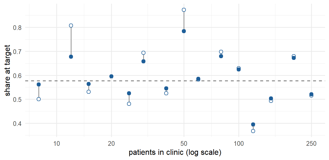
Plot how far each clinic moves (no pooling minus partial pooling) against its number of patients.

Solution

fit_complete <- brm(at_target | trials(n_patients) ~ 1, family = binomial(),
                    prior = prior(normal(0, 1.5), class = "Intercept"),
                    data = clinics, chains = 4, iter = 2000, seed = 530, refresh = 0)
fit_none <- brm(at_target | trials(n_patients) ~ 0 + clinic, family = binomial(),
                prior = prior(normal(0, 1.5), class = "b"),
                data = clinics, chains = 4, iter = 2000, seed = 530, refresh = 0)
fit_partial <- brm(at_target | trials(n_patients) ~ 1 + (1 | clinic), family = binomial(),
                   prior = c(prior(normal(0, 1.5), class = "Intercept"),
                             prior(exponential(1), class = "sd")),
                   data = clinics, chains = 4, iter = 2000, seed = 530, refresh = 0)

share_none    <- colMeans(posterior_linpred(fit_none, transform = TRUE))
share_partial <- colMeans(posterior_linpred(fit_partial, transform = TRUE))
share_complete <- mean(plogis(as_draws_df(fit_complete)$b_Intercept))
comparison <- data.frame(clinic = clinics$clinic, n_patients = clinics$n_patients,
                         observed = clinics$at_target / clinics$n_patients,
                         no_pooling = share_none, partial_pooling = share_partial,
                         complete_pooling = share_complete)
comparison$shift <- comparison$no_pooling - comparison$partial_pooling
ggplot(comparison, aes(n_patients, abs(shift))) + geom_point() + scale_x_log10()

What we got (partial-pooling model): sd(Intercept) = 0.76 (95% CrI 0.46–1.22), Intercept 0.35, so the average clinic has about plogis(0.35) ≈ 59% at target. Rhat 1.00, ESS > 600.

Clinic	Patients	Observed	No pooling	Partial pooling	Complete pooling
A	8	0.875	0.79	0.72	0.57
B	12	0.917	0.85	0.77	0.57
H	50	0.280	0.29	0.32	0.57
K	100	0.340	0.34	0.36	0.57
O	250	0.760	0.76	0.75	0.57

The two smallest clinics move by about 0.07 between no and partial pooling; the four largest by less than 0.01. Note that even the no-pooling estimates for A and B lie below the observed shares: their normal(0, 1.5) prior on the log-odds pulls each clinic towards 0.5, not towards the other clinics. That is a fixed prior, not pooling.

Task 5.2 · Ranks with uncertainty

Rank the 15 clinics by share at target in every posterior draw of the partial-pooling model. Report each clinic’s mean rank, a 95% interval for the rank and the probability of being in the top 3.

Solution

share_draws <- posterior_linpred(fit_partial, transform = TRUE)
rank_draws  <- t(apply(-share_draws, 1, rank))            # rank 1 = best
colnames(rank_draws) <- clinics$clinic
rank_summary <- data.frame(clinic = clinics$clinic,
                           mean_rank = colMeans(rank_draws),
                           lower_95 = apply(rank_draws, 2, quantile, 0.025),
                           upper_95 = apply(rank_draws, 2, quantile, 0.975),
                           prob_top3 = colMeans(rank_draws <= 3))
rank_summary[order(rank_summary$mean_rank), ]

What we got: B and O share the best mean rank (2.7) and have the highest probabilities of being in the top 3 (0.72 and 0.74). But B’s 95% rank interval is 1–8 (12 patients) while O’s is 1–5 (250 patients). A (8 patients) could be anywhere from 1st to 11th. H and K are almost certainly among the bottom four (intervals 12–15). A league table would show B and O as “joint best” and hide the difference in certainty.

Task 5.3 · A clinic you have not seen yet

Predict the number at target out of 100 patients (a) for a new clinic and (b) for existing clinic O. Then do it the wrong way: plug in the posterior means of the intercept and τ. Compare the three 90% intervals.

Solution

new_clinic <- data.frame(clinic = "new", n_patients = 100)
quantile(posterior_epred(fit_partial, newdata = new_clinic, allow_new_levels = TRUE,
                         sample_new_levels = "gaussian"), c(0.05, 0.5, 0.95))
existing <- data.frame(clinic = "O", n_patients = 100)
quantile(posterior_epred(fit_partial, newdata = existing), c(0.05, 0.5, 0.95))

draws_partial <- as_draws_df(fit_partial)
plugin_share <- plogis(mean(draws_partial$b_Intercept) +
                       rnorm(4000, 0, mean(draws_partial$sd_clinic__Intercept)))
quantile(100 * plugin_share, c(0.05, 0.5, 0.95))

What we got (number at target out of 100):

	Median	90% interval
New clinic	58	27–85
Existing clinic O	76	71–80
New clinic, plug-in of posterior means	59	30–84

A new clinic is far more uncertain than O, whose own 250 patients pin it down. The plug-in interval is slightly too narrow because it ignores the uncertainty in μ and τ. With 15 clinics τ is fairly well estimated, so the difference is small here. With few groups it would be much larger.

Task 5.4 · Varying intercepts and slopes: blood pressure over five monthly visits

set.seed(531)
sd_intercept <- 10; sd_slope <- 1.5; cor_intercept_slope <- -0.4
cov_matrix <- matrix(c(sd_intercept^2, cor_intercept_slope * sd_intercept * sd_slope,
                       cor_intercept_slope * sd_intercept * sd_slope, sd_slope^2), nrow = 2)
patient_effects <- MASS::mvrnorm(40, mu = c(0, 0), Sigma = cov_matrix)
bp <- expand.grid(month = 0:4, patient = 1:40)
bp$sbp <- 150 + patient_effects[bp$patient, 1] +
          (-2 + patient_effects[bp$patient, 2]) * bp$month + rnorm(nrow(bp), 0, 5)

Fit sbp ~ month + (1 + month | patient) with priors normal(150, 20) (Intercept), normal(0, 5) (b), exponential(0.2) (sd and sigma) and lkj(2) (cor). Do you recover the simulated values?
Compute, per draw, the share of patients whose own slope is negative. Why is this not simply pnorm(0, b_month, sd_month)?

Solution

fit_slopes <- brm(sbp ~ month + (1 + month | patient), family = gaussian(),
                  prior = c(prior(normal(150, 20), class = "Intercept"),
                            prior(normal(0, 5), class = "b"),
                            prior(exponential(0.2), class = "sd"),
                            prior(exponential(0.2), class = "sigma"),
                            prior(lkj(2), class = "cor")),
                  data = bp, chains = 4, iter = 2000, seed = 531, refresh = 0)
summary(fit_slopes)

draws_slopes <- as_draws_df(fit_slopes)
slope_columns <- grep("^r_patient\\[.*,month\\]$", names(draws_slopes), value = TRUE)
patient_slopes <- draws_slopes$b_month + as.matrix(draws_slopes[, slope_columns])
quantile(rowMeans(patient_slopes < 0), c(0.05, 0.5, 0.95))

What we got: sd(Intercept) 10.5 (simulated 10), sd(month) 1.53 (simulated 1.5), month −1.91 (simulated −2), sigma 4.87 (simulated 5), all Rhat ≤ 1.01. The correlation is −0.23 with a 95% interval from −0.60 to 0.24 (simulated −0.4): correlations of varying effects need many groups to be estimated precisely.

Share of the 40 patients with a negative own slope: median 0.90 (90% interval 0.80–1.00). pnorm(0, b_month, sd_month) answers a different question: the share in the population of patients (about 0.89 here). The first is about these 40 patients and uses their data; the second is about future patients. Both are legitimate estimands; say which one you report.

Task 5.5 · How much does the hyperprior matter with few groups?

Keep only six clinics (few_clinics <- clinics[clinics$clinic %in% c("A", "C", "E", "G", "I", "K"), ]) and fit the partial-pooling model twice: with exponential(1) and with exponential(0.1) on the SD (control = list(adapt_delta = 0.95)). Compare the posteriors of τ.

Solution

fit_tau_exp1 <- brm(at_target | trials(n_patients) ~ 1 + (1 | clinic), family = binomial(),
                    prior = c(prior(normal(0, 1.5), class = "Intercept"),
                              prior(exponential(1), class = "sd")),
                    data = few_clinics, chains = 4, iter = 2000, seed = 532, refresh = 0,
                    control = list(adapt_delta = 0.95))
fit_tau_exp01 <- brm(at_target | trials(n_patients) ~ 1 + (1 | clinic), family = binomial(),
                     prior = c(prior(normal(0, 1.5), class = "Intercept"),
                               prior(exponential(0.1), class = "sd")),
                     data = few_clinics, chains = 4, iter = 2000, seed = 532, refresh = 0,
                     control = list(adapt_delta = 0.95))
rbind(exponential_1   = posterior_summary(fit_tau_exp1,  variable = "sd_clinic__Intercept"),
      exponential_0.1 = posterior_summary(fit_tau_exp01, variable = "sd_clinic__Intercept"))

What we got:

Hyperprior on τ	Posterior mean τ	95% interval
`exponential(1)`	0.70	0.20–1.60
`exponential(0.1)`	0.88	0.23–2.30

With six clinics the lower part of τ’s posterior is set by the data, but the upper tail follows the prior: 1.6 vs 2.3 on the log-odds scale is the difference between “clinics differ by up to an odds ratio of about 5 (one SD)” and “about 10”. Report τ with a hyperprior sensitivity analysis whenever the number of groups is small, as with Sweden’s 8 regions in the project.

Why-questions

Why do the most extreme raw estimates usually come from the smallest groups?

Small groups have large sampling variance, so their observed rates scatter widely around their true rates. The extremes of a noisy list are mostly noise. Partial pooling pulls them back in proportion to their noise.

Why can’t the no-pooling model predict a new hospital?

It has a separate parameter for each observed hospital and no distribution connecting them. A new hospital has no parameter and nothing to draw one from. The hierarchical model supplies $N(\mu, \tau^2)$.

Why is a hierarchical model “Bayesian” even when fitted with lme4?

The group effects get a distribution whose parameters are estimated from the data: a prior learned from the other groups. lme4 estimates μ and τ by (restricted) maximum likelihood and plugs them in, much like empirical Bayes; brms also integrates over their uncertainty.

Spaced review: Modules 1–4

1. What does the shrinkage formula from Module 2 have in common with partial pooling?

Both pull an estimate towards a prior mean by a fraction (sampling variance)/(sampling variance + prior variance). In a hierarchical model the “prior” is the estimated population distribution. (2.3)

2. How would you check whether a random intercept for region is needed?

Posterior predictive check of the region means (stat_grouped by region) for the model without it, and loo_compare with and without the term; think about grouped CV if the question is about new regions. (4.3, 4.8)

3. A varying-slopes model gives 30 divergent transitions. First step?

Increase adapt_delta (e.g. 0.99); if they persist, tighten the priors on the SDs and correlation or simplify the random-effect structure. Divergences can bias the estimates. (3.7)