Module 6 — Bayesian Workflow and Open Problems

The iterative workflow · prior predictive checks · temporal coherence · weakly informative priors · sensitivity analysis · calibration · “objective” priors · subjectivity

Module 1 described the Bayesian analysis in four tidy steps: model, prior, posterior, evaluation. Real analyses never run in a straight line. A posterior predictive check fails and you change the likelihood; the chains do not converge and you simplify the model or tighten a prior; a prior predictive check shows the prior allows absurd data and you rethink it. Module 6 is about doing this loop well and honestly. It is also the blueprint for your project.

The main new tool is the prior predictive check: simulate data from the prior alone, before looking at the data, and see whether the prior implies plausible outcomes. It is the easiest way to make sense of priors in many dimensions, where the joint effect of individually “vague” priors can be surprisingly extreme, especially through a link function.

The module then turns to open problems. Every time the data make you change the model or the prior, you use the data twice, which breaks temporal coherence. What counts as a “good” prior: one with good frequentist properties (calibration), one with mathematical invariance (Jeffreys, reference priors), or one that honestly encodes expert knowledge? And is Bayesian statistics more “subjective” than classical statistics? The syllabus asks you to discuss these questions, so there is no single right answer to memorise. The aim is a defensible position.

Sources, reading and lecture

Course notes: Module 6 “Bayesian Workflow and other Open Problems” (pp. 263–287). There is a lecture on Bayesian workflow in October; check TimeEdit.

Key reference: Gelman, Vehtari, Simpson et al. (2020), “Bayesian Workflow”, arXiv:2011.01808. Gabry et al. (2019), “Visualization in Bayesian workflow”, JRSS A (prior predictive checks). Talts et al. (2018), “Validating Bayesian inference algorithms with simulation-based calibration”.

Examples on this page (vaccination priors, a calibration simulation) are written for this app.

Before you start: three things you need

Posterior predictive check (4.2): simulate replicated data from the posterior and compare with the observed data. A prior predictive check does the same with the prior.

The logit link. \(p = \text{plogis}(\eta)\). \(\eta = \pm 5\) already means \(p \approx 0.007\) or \(0.993\). A normal(0, 10) prior on \(\eta\) puts most of its mass beyond ±5.

Coverage (2.8): the share of intervals that contain the true value over repeated experiments.

Part A · Concepts

6.1 The workflow is iterative

The four steps from Module 1, with the loops that real analyses need:

  ┌──────────────────────────────────────────────────────────────┐
  │ 1. Model: likelihood + structure for everything (data, θ)   │◀──────────┐
  └──────────────────────────────┬───────────────────────────────┘           │
  ┌──────────────────────────────▼───────────────────────────────┐           │
  │ 2. Prior ── prior predictive check ── absurd? change prior ─┼──┐        │
  └──────────────────────────────┬───────────────────────────────┘  │ still  │
  ┌──────────────────────────────▼───────────────────────────────┐  │ absurd?│
  │ 3. Fit: MCMC ── converged? (R-hat, ESS, divergences) ── no ─┼──┴────────┤
  └──────────────────────────────┬───────────────────────────────┘           │
  ┌──────────────────────────────▼───────────────────────────────┐           │
  │ 4. Check: posterior predictive checks, LOO ── misfit? ──────┼───────────┘
  └──────────────────────────────┬───────────────────────────────┘
  ┌──────────────────────────────▼───────────────────────────────┐
  │ 5. Several plausible models? compare, stack, or report all  │
  │ 6. Sensitivity: priors, model choices                        │
  │ 7. Estimands from the draws → tables, figures, conclusions   │
  └──────────────────────────────────────────────────────────────┘

Gelman et al. (2020) list many more steps, including “add more data” and “give up”: not every question can be answered with the data at hand. Two practical habits make the loop manageable:

Start simple and build up: an intercept-only model, then covariates, then group effects, then varying slopes. When something breaks, you know which addition broke it.
Keep a log of every model you fit and why you changed it. You need it for the methods section anyway (Section 6.3).

6.2 Prior predictive checks

Simulate data from the prior alone: draw parameters from the prior, plug them into the likelihood, look at the simulated outcomes. In brms, add sample_prior = "only" to brm(), then use pp_check() and posterior_predict() exactly as for the posterior.

What to look for:

The prior predictive should cover every outcome that is plausible: previously observed ranges, theoretically possible values.
It should not put much mass on implausible outcomes: negative lengths of stay, blood pressures of 900, a 100% or 0% prevalence in every population.
It is not supposed to reproduce your data. That would mean you tuned the prior on the data (Section 6.3).

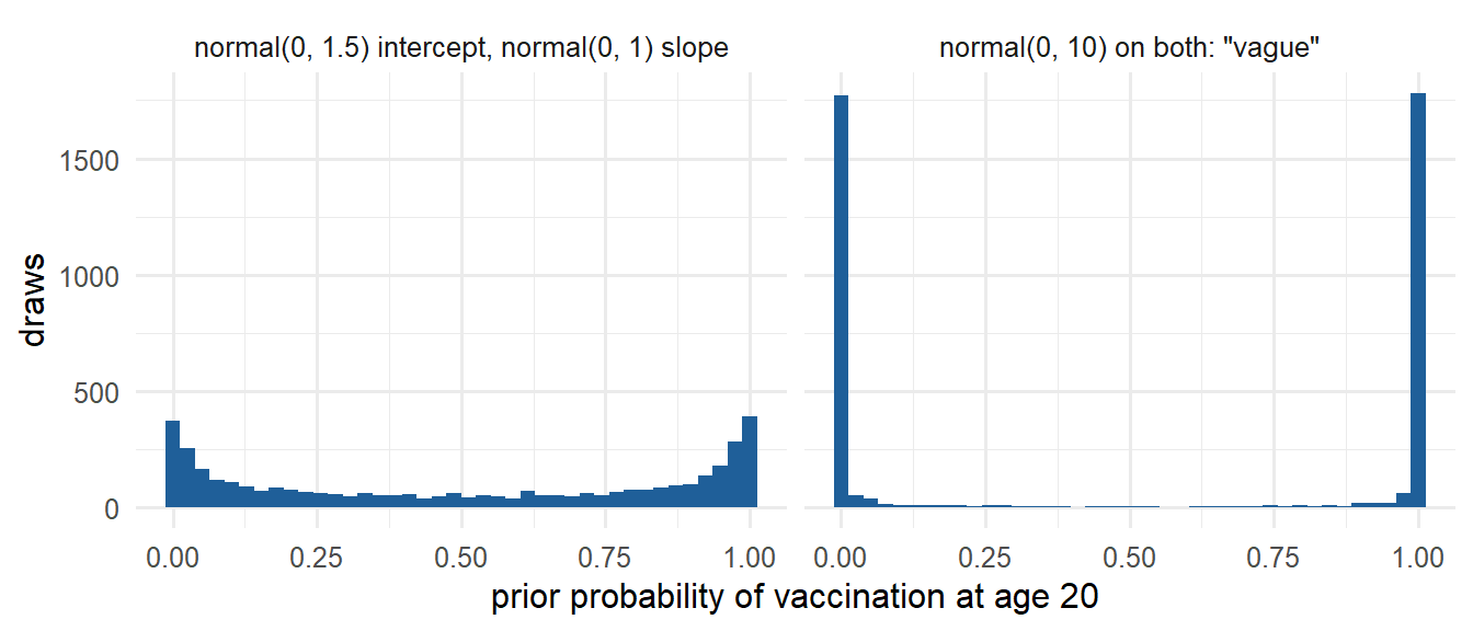
Figure 1: Implied probability of vaccination at age 20 under two priors for a logistic regression (intercept and slope per decade, age centred at 50). Each histogram shows 4,000 prior draws.

The “vague” prior is not vague at all on the probability scale: it says almost every 20-year-old population is either nearly all vaccinated or nearly all unvaccinated (the U shape). Priors that look weak on the linear-predictor scale can be strongly informative on the outcome scale once they pass through a link function or are combined across many coefficients.

Common confusion: “a flat or very wide prior is the safe, neutral choice”

A flat prior on a coefficient says an odds ratio of \(10^6\) is as plausible as 1.5. Flat priors can also give improper posteriors or poor convergence. A weakly informative prior that rules out absurd values is usually safer. A prior predictive check shows what each prior actually implies.

Nothing, since priors should always be vague

Tighten or rescale the priors until simulated weights are plausible

Tune the prior until it reproduces the observed weights exactly

Switch to a flat prior, which cannot produce impossible values

The prior implies impossible data, so revise it (or the likelihood, e.g. a log-normal for a positive outcome). Tuning the prior to reproduce the observed data uses the data twice. A flat prior makes the problem worse.

6.3 Temporal coherence: using the data twice

Strict Bayesian updating says: specify the prior before seeing the data, and never revisit it. Every time a check on the data makes you widen a prior or add a term, the “prior” of the final model has been informed by the data, which is then used again to compute the posterior. The notes (following David Cox) call this a loss of temporal coherence.

Changing the model after a failed posterior predictive check is equivalent to changing the prior on an extra coefficient from “exactly zero” to something weaker, using the data.
It is not a Bayesian problem only: stepwise variable selection, choosing among many models, and choosing covariates after looking at results all make classical p-values and intervals too optimistic.
It is not a reason to keep a model you know is wrong. Cox: hypotheses generated by the data are not worthless, but they are “in some way distinct from hypotheses considered a priori”, and cannot be trusted as much as a test on fresh data.

What to do in practice:

Plan as much as possible before looking at outcomes: research question, estimand, model family, priors, planned checks. For found data (like survey data) this is harder but still possible.
Report every model fitted and every change made, and why.
Temper your conclusions for data-driven choices; present them as hypotheses for new data.

6.4 Weakly informative priors

Between flat priors and fully elicited expert priors lies the practical default: priors that rule out absurd values but say little else.

Parameter	Think about	Typical weakly informative choice
Log odds ratio / logistic slope	ORs above 20 or below 1/20 per unit are rare in health research	`normal(0, 1)` to `normal(0, 2.5)`, after scaling the predictor
Intercept (logistic)	the baseline probability: roughly between 1% and 99%?	`normal(0, 1.5)` (or centred on a known prevalence)
Slope in a linear model	the outcome range and the predictor’s units	normal with SD ≈ (plausible outcome range) / (predictor range)
Residual SD \(\sigma\)	the outcome’s scale	`exponential(1 / typical SD)` or half-normal
Group-level SD \(\tau\)	how different groups could be	`exponential(1)` to `exponential(2)` on the logit scale
Correlation matrix		`lkj(2)`

Scaling helps. Priors are easier on centred and standardised predictors, or on meaningful units: age in decades, income in quintiles. The notes: scientists choose units so that effects are small numbers; “the bulk of the prior mass should lie in a range of small numbers”.

brms defaults (see get_prior()): flat on regression coefficients, Student-t on the intercept and SDs, scaled to the data. The notes call defaults “not great, not terrible”: better than nothing, but not a substitute for thinking, and the fact that a default worked ten times does not mean it works the eleventh.

6.5 Prior sensitivity analysis

Show how much the conclusions depend on the priors:

Fit the main analysis with your chosen priors.
Refit with alternatives: wider, narrower, differently centred (for example a sceptical prior centred on no effect), a different family for SDs.
Report the estimand under each. If the conclusions agree, say so. If they do not, the data alone cannot settle the question, and that is a finding to report.

Most informative are priors for parameters the data say little about: group-level SDs with few groups, coefficients of rare exposures, interactions. The same logic applies to model choices: normal vs Student-t, with or without a random slope. The priorsense package (power-scaling sensitivity) automates part of this for brms fits.

Compare prior and posterior for key parameters: a posterior identical to the prior means the data are uninformative about that parameter.

6.6 Calibration: frequentist properties of Bayesian procedures

How good is a prior? Borrow classical criteria (bias, coverage, efficiency) and study them by simulation:

Choose a data-generating mechanism and true parameter values (several settings, some unfavourable).
Simulate many datasets; fit the model with the chosen prior to each.
Record bias of the posterior mean, coverage of the credible intervals, and interval width.

What to expect: a prior centred on the truth over-covers; one centred ±2 prior SDs away under-covers (2.8). A reasonable hope is good coverage on average over plausible true values.

Simulation-based calibration (SBC). Draw the true value from the prior itself, simulate data, fit, and compute where the true value falls in its posterior (its posterior quantile). If model, prior and software are all correct, these quantiles are uniform and the 95% intervals cover 95% of the time on average. Stan’s developers use this to test the software. A non-uniform histogram reveals a bug or a mismatch between the prior used for generating and for fitting.

6.7 “Objective” priors

Attempts to define priors by mathematical principle rather than knowledge:

Flat priors. Not invariant: flat on \(\sigma\) is not flat on \(\sigma^2\) or \(\log\sigma\). If \(X \sim \text{Uniform}(7, 22)\), then \(X^2\) is not uniform on \((49, 484)\).
Jeffreys’ prior, \(p(\theta) \propto \sqrt{I(\theta)}\) (Fisher information). Invariant under reparameterisation: you get the same answer whether you work with \(\theta\) or \(\theta^2\). Examples: flat for a normal mean with known variance; \(\text{Beta}(\tfrac12, \tfrac12)\) for a binomial proportion; \(1/\sigma\) for a normal SD. Critiques: depends on the likelihood (so two analysts with different models get different “non-informative” priors), and multi-parameter versions are controversial.
Reference priors maximise the expected KL divergence between prior and posterior: they let the data dominate as much as possible. In one dimension they usually coincide with Jeffreys’.
Priors that mimic frequentist results (probability matching), shrinkage priors for sparsity (spike-and-slab, horseshoe), and penalised complexity (PC) priors that favour the simpler model. These are active research areas.

None has settled the question: “objective” priors are conventions that other analysts can reproduce.

6.8 Subjectivity in Bayesian and non-Bayesian workflows

The syllabus asks you to discuss subjectivity in data collection, prior specification and model specification. The notes’ main points:

Every analysis is full of choices: research question, data source, inclusion criteria, variables, model family, functional form, how to handle outliers and missing data, what to report. In a classical analysis many of these are implicit. Choosing not to use a prior is also a choice.
The prior is often the least dangerous choice: it is explicit, can be checked with prior predictive checks and varied in a sensitivity analysis. Its influence fades with more data (though not with more parameters: in genomics, with many small clusters or with \(p \gg n\), priors stay influential).
Informative priors can be more accurate. The German tank problem in Module 1 of the notes and the fish example in Module 1 here: a well-reasoned prior plus little data beats little data alone.
“Objective” may really mean transparent and reproducible: report every step so others could reproduce it or vary it (Draper’s “transparent subjectivity”).
Eliciting priors from experts is a skill. Experts’ priors disagree, are often overconfident, and eliciting them costs time; facilitation protocols exist. In practice defaults and weakly informative priors fill the gap.
The statistician’s role. Priors are where domain experts can contribute directly without knowing MCMC. The notes imagine collaborators debating priors and predictive checks instead of p-values.

Discussion prompts for the seminar or the project report

Name three subjective choices in a classical analysis of your project data that a reader might not notice.
Your collaborator says “Bayesian results are just your opinion”. Give a two-sentence reply using the fish example or a sensitivity analysis.
When would you prefer a sceptical prior over a weakly informative one? Who should decide?
You changed the model after a failed posterior predictive check. How do you report that honestly?

When to use these tools

Prior predictive checks: for every model with non-trivial priors, especially GLMs and GLMMs where link functions distort vague priors.
Sensitivity analysis: for every published analysis; essential for group-level SDs with few groups and for parameters the data barely inform.
Calibration / SBC: when you write a new model or custom Stan code, or want to know how a prior behaves under repeated use.

Limitations

Prior predictive checks only reveal absurd marginal implications that you think to look at; a prior can pass them and still be poor.
Sensitivity analyses can only vary what you think of varying.
There is no agreed definition of an “objective” prior, and a fully coherent workflow is rarely achievable with found data.

Part B · Practice

In the browser

Interactive R

Runs in your browser; no data needed.

Exercise 1 · A prior predictive check by hand. Logistic regression for vaccination by age (age in decades from 50).

Why is the share of extreme probabilities lower at age 50 than at ages 20 and 80?
Try implied_probabilities(1.5, 0.5). Is a slope SD of 0.5 per decade reasonable for vaccination uptake?

Model answer

At age 50, age10 = 0, so only the intercept matters. At 20 and 80 the slope is multiplied by ±3, so its prior spread is tripled on the log-odds scale. With the wide prior about 88% of draws are extreme at ages 20 and 80, and still 65% at age 50.
SD 0.5 per decade means an odds ratio per decade mostly between \(e^{-1} \approx 0.37\) and \(e^{1} \approx 2.7\), and across 30 years between about 0.05 and 20. Plausible for uptake that rises strongly with age, without absurd values. Whether it is “right” is a subject-matter question.

Exercise 2 · Simulation-based calibration of a Beta–Binomial model.

Explain the shape of the second histogram. In which direction are the posteriors wrong?
Fit with a flat prior (a_fit = 1, b_fit = 1) while generating from Beta(2, 2). Is it calibrated? Why is that not a contradiction?

Model answer

Most true values fall in the lowest part of their posteriors: the Beta(8, 2) prior pulls every posterior upwards, so the truth sits in the lower tail. Coverage drops to about 0.71 instead of 0.95.
Close to uniform, coverage about 0.95. With 20 observations the flat prior lets the data dominate, and it does not pull in a systematically wrong direction. Calibration “on average” does not require the fitting prior to equal the generating one, but mismatch in location, as in Question 3, shows up quickly.

In RStudio: brms tasks

How the RStudio tasks work

The data are simulated in the script (the same vaccination data as Task 4.2). Download: module6-tasks.R.

Task 6.1 · Prior predictive check with sample_prior = "only"

Fit vaccinated ~ age10 twice with sample_prior = "only": once with normal(0, 10) on both intercept and slope, once with normal(0, 1.5) (Intercept) and normal(0, 1) (b).

Compare pp_check(fit, type = "stat", stat = "mean") for the two priors.
What share of prior draws implies an overall vaccination share below 5% or above 95%?
What share of prior draws implies a probability below 1% at age 20?

Solution

prior_wide <- brm(vaccinated ~ age10, family = bernoulli(),
                  prior = c(prior(normal(0, 10), class = "Intercept"),
                            prior(normal(0, 10), class = "b")),
                  data = vaccine, sample_prior = "only",
                  chains = 4, iter = 1000, seed = 610, refresh = 0)
prior_weak <- brm(vaccinated ~ age10, family = bernoulli(),
                  prior = c(prior(normal(0, 1.5), class = "Intercept"),
                            prior(normal(0, 1), class = "b")),
                  data = vaccine, sample_prior = "only",
                  chains = 4, iter = 1000, seed = 610, refresh = 0)
pp_check(prior_wide, type = "stat", stat = "mean")
pp_check(prior_weak, type = "stat", stat = "mean")

prior_share_wide <- rowMeans(posterior_predict(prior_wide))
prior_share_weak <- rowMeans(posterior_predict(prior_weak))
c(mean(prior_share_wide < 0.05 | prior_share_wide > 0.95),
  mean(prior_share_weak < 0.05 | prior_share_weak > 0.95))

extreme_ages <- data.frame(age10 = c(-3, 3))
c(mean(posterior_epred(prior_wide, newdata = extreme_ages)[, 1] < 0.01),
  mean(posterior_epred(prior_weak, newdata = extreme_ages)[, 1] < 0.01))

What we got: the overall share looks less alarming than you might expect: 19% of the wide-prior draws imply an overall vaccination share below 5% or above 95%, against 2% for the weak prior. With a steep prior slope, young people end up near 0 and old people near 1, so the average lands in the middle. The overall mean hides the problem, and brms even warns that “mean” is a weak statistic.

At a specific age the difference is stark: 47% of wide-prior draws put the probability of vaccination at age 20 below 1%, against 11% for the weak prior. Check prior implications at the covariate values that matter, not only overall.

Task 6.2 · Prior sensitivity: does the conclusion change?

Refit both models to the data (update(prior_weak, sample_prior = "no")) and compare the posterior of the age slope. What does the comparison tell you, and when would you expect a larger difference?

Solution

fit_weak <- update(prior_weak, sample_prior = "no", seed = 611, refresh = 0)
fit_wide <- update(prior_wide, sample_prior = "no", seed = 611, refresh = 0)
rbind(weak = posterior_summary(fit_weak, variable = "b_age10"),
      wide = posterior_summary(fit_wide, variable = "b_age10"))

What we got: b_age10 = 0.503 (SD 0.044) with the weak prior and 0.505 (SD 0.045) with the wide prior. Practically identical: 800 people inform one slope far more than either prior does.

Expect priors to matter more with few observations or few events, group-level SDs with few groups (Task 5.5), many coefficients relative to the data, and separation (a covariate predicts the outcome perfectly, so the likelihood keeps increasing towards infinite coefficients and only the prior stops it). A prior predictive check is worth doing even when the posterior turns out insensitive, because you do not know in advance which case you are in.

Why-questions

Why check the prior on the outcome scale rather than the parameter scale?

Priors on individual parameters combine (and pass through link functions) in ways that are hard to foresee. The outcome scale is where domain knowledge lives: experts know plausible blood pressures and prevalences, not plausible log odds ratios.

Why is revising a model after a failed check still better than keeping it?

A model known to be wrong gives conclusions known to be unreliable. Revising uses the data twice, which makes the final uncertainty somewhat optimistic; reporting the revision lets readers judge that.

Why doesn’t more data make priors irrelevant in hierarchical models?

Adding observations within existing groups sharpens each group’s estimate, but τ is informed by the number of groups. More groups add parameters too, so the ratio of parameters to data does not go to zero, and priors on group-level quantities stay influential.

Spaced review: Modules 1–5

1. What does a posterior predictive p-value of 0.98 for the maximum mean?

Replicated maxima are almost always larger than the observed maximum: the model predicts heavier upper tails than the data show. (4.3)

2. Why is a new group’s prediction wider than an existing group’s?

It adds a draw of the group effect from N(0, τ²), with τ itself uncertain; an existing group’s effect is informed by its own data. (5.6)

3. Which is the syllabus-listed learning outcome for Module 3?

Explain the challenge of convergence in distribution of the MCMC sample to the true posterior and list common causes of failure to converge (poor identification, multimodality, too short warm-up, strong autocorrelation, bad parameterisation). (3.8)