Module 2 — Continuous Priors: Conjugate Distributions
Densities and grids · normal–normal and shrinkage · sequential updating · Beta–Binomial · prior as data · posterior predictive · Gamma–Poisson · why conjugacy runs out
In Module 1 the parameter could only take a list of values, so Bayes’ rule needed a sum. Most parameters are continuous (a mean, a proportion, a rate), and then the denominator of Bayes’ rule is an integral. Integrals are hard in general. This module covers the special cases where they are easy.
A prior is conjugate to a likelihood when the posterior belongs to the same family as the prior. Then updating is just arithmetic on the prior’s parameters: a Beta prior plus binomial data gives a Beta posterior, a Gamma prior plus Poisson counts gives a Gamma posterior, and a normal prior plus normal data with known variance gives a normal posterior.
Conjugate models show the logic of Bayesian inference with nothing hidden. The posterior mean is a compromise between the prior mean and the data, weighted by how informative each is. Precision adds up. The prior behaves like extra data with an equivalent sample size. The data are “shrunk” towards the prior, and this shrinkage returns in Module 5 as partial pooling.
Conjugacy runs out quickly. The list of conjugate pairs is short, and realistic models (Student-t errors, detection limits, several unknown parameters) leave it. That is the motivation for MCMC in Module 3.
NoteSources, reading and seminar
Course notes: Module 2 “Continuous priors: conjugate distributions” (pp. 53–96). Reading deadline: Seminar 2, Monday 14 September 2026.
Optional textbook: McElreath, Statistical Rethinking, chapters 2–4 (grid approximation, the normal model).
Examples on this page (a patient’s HbA1c, medication adherence, ward infection rates) are written for this app. The course notes use other examples.
TipBefore you start: three things you need
Density vs mass. For a continuous variable, \(p(x)\) is a density: probabilities are areas, \(P(a < X < b) = \int_a^b p(x)\,dx\), and \(p(x)\) itself can exceed 1.
Precision. Precision = 1 / variance. A normal distribution with SD 2 has precision 0.25.
Kernel. The part of a density that depends on the variable. \(\text{Beta}(a, b) \propto \theta^{a-1}(1-\theta)^{b-1}\); the constant in front only makes it integrate to 1. Recognising a kernel is how conjugate posteriors are derived: drop constants, multiply, and see which family appears.
Part A · Concepts
2.1 From sums to integrals, and back to sums
For a continuous parameter,
\[p(\theta \mid y) = \frac{p(y \mid \theta)\, p(\theta)}{\int p(y \mid \theta)\, p(\theta)\, d\theta}.\]
The denominator is only a normalising constant: it makes the posterior integrate to 1. Two ways around it:
- Calculus. For conjugate pairs the integral has a known answer: recognise the kernel of the posterior.
- Approximate the integral by a sum (a Riemann sum). Evaluate prior × likelihood on a fine grid of \(\theta\) values, then divide by the sum times the grid width. This is exactly the Module 1 recipe, and it works well for one or two parameters.
A histogram of a large sample is the same idea in reverse: with enough draws and narrow bins it traces out the density. That is why a sample of posterior draws (Module 3) can stand in for the posterior itself.
2.2 Normal data with known variance: precision adds up
Data \(y_1, \dots, y_n \sim N(\mu, \sigma^2)\) with \(\sigma\) known, prior \(\mu \sim N(\mu_0, \sigma_0^2)\). The posterior is normal with
\[\frac{1}{\sigma_n^2} = \underbrace{\frac{1}{\sigma_0^2}}_{\text{prior precision}} + \underbrace{\frac{n}{\sigma^2}}_{\text{data precision}}, \qquad \mu_n = \frac{\frac{1}{\sigma_0^2}\mu_0 + \frac{n}{\sigma^2}\bar y}{\frac{1}{\sigma_0^2} + \frac{n}{\sigma^2}}.\]
- Precision adds: the posterior is always more precise than both the prior and the data alone, even if the data conflict with the prior.
- The posterior mean is a precision-weighted average of the prior mean and the sample mean.
- Only \(\bar y\) enters: it is a sufficient statistic here.
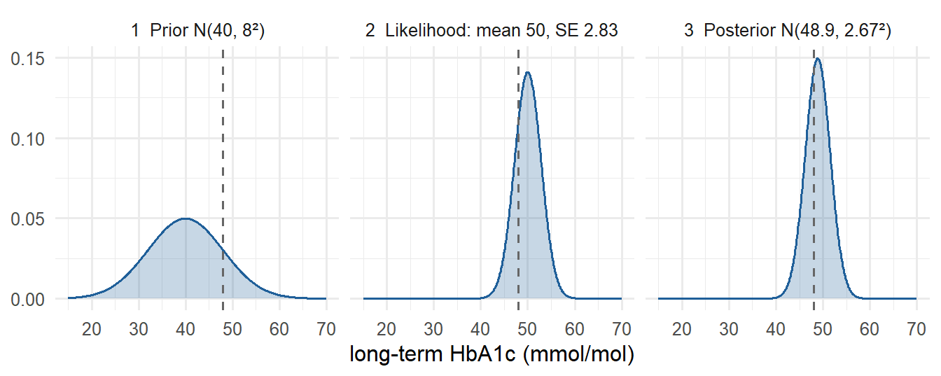
Worked example: a patient’s long-term HbA1c. Two measurements average \(\bar y = 50\) mmol/mol. Measurement variation (analytical + biological) is \(\sigma = 4\). In the patient’s age group, long-term HbA1c has mean 40 and SD 8; use that as the prior, \(N(40, 8^2)\).
| Precision | Mean | SD | 95% interval | |
|---|---|---|---|---|
| Prior | 1/64 = 0.016 | 40 | 8 | |
| Data (2 readings) | 2/16 = 0.125 | 50 | 2.83 | classical CI 44.5–55.5 |
| Posterior | 0.141 | 48.9 | 2.67 | credible 43.7–54.1 |
The posterior mean moved 1.1 units towards the population mean. The two readings are fairly precise, so the move is small. The diagnostic threshold for diabetes is 48 mmol/mol, and the posterior answers the clinical question directly: \(P(\mu > 48 \mid y) = 0.63\).
It moves further towards the prior mean 40
It moves closer to 50 and becomes narrower
It stays at 48.9 but becomes narrower
It becomes wider, since more data add variance
Data precision becomes 8/16 = 0.5, much larger than the prior precision 0.016. The weight on ȳ grows, so the mean moves towards 50 (about 49.7), and the total precision grows, so the SD shrinks (about 1.4).
2.3 Shrinkage: three ways to write the same posterior mean
\[\mu_n = \underbrace{w\,\mu_0 + (1-w)\,\bar y}_{\text{weighted average}} = \underbrace{\mu_0 + (\bar y - \mu_0)\frac{\sigma_0^2}{\sigma_0^2 + \sigma^2/n}}_{\text{prior adjusted towards the data}} = \underbrace{\bar y - (\bar y - \mu_0)\frac{\sigma^2/n}{\sigma^2/n + \sigma_0^2}}_{\text{data shrunk towards the prior}}\]
with \(w = \dfrac{1/\sigma_0^2}{1/\sigma_0^2 + n/\sigma^2}\).
The last form is shrinkage: the estimate is pulled from \(\bar y\) towards \(\mu_0\), and the fraction pulled is (sampling variance of \(\bar y\)) / (sampling variance + prior variance). Noisy data, or a confident prior, means more shrinkage.
Limits: \(\mu_n = \mu_0\) if \(\sigma_0^2 = 0\) (a prior certain of \(\mu_0\)); \(\mu_n = \bar y\) if \(\sigma^2 = 0\) or \(\sigma_0^2 \to \infty\).
Intuition from the HbA1c example: a patient measured higher than typical for their age. Part of that may be chance (two readings happened to be high), so the best estimate of their long-term value is slightly lower than their measured mean. With more readings, the chance explanation becomes less plausible and the shrinkage disappears. Module 5 applies exactly this to groups: small hospitals’ rates are shrunk towards the average hospital.
2.4 Flat priors, improper priors and the classical interval
Let \(\sigma_0^2 \to \infty\): the prior becomes flat over the whole real line. The posterior becomes \(N(\bar y, \sigma^2/n)\), and the 95% credible interval is \(\bar y \pm 1.96\,\sigma/\sqrt n\): numerically identical to the classical confidence interval, though still interpreted as a probability statement about \(\mu\).
- A flat prior on the real line is improper: it does not integrate to 1. Here the posterior is still proper, but that is not guaranteed in general. An improper posterior cannot be used.
- “Non-informative” is misleading. A flat prior says that \(\mu\) between 1 and 2 million is exactly as plausible as \(\mu\) between 1 and 2. That is rarely anybody’s actual belief.
- Flat on one scale is not flat on another: flat on \(\sigma\) is not flat on \(\sigma^2\) or \(\log \sigma\) (Module 6).
2.5 Sequential updating
Today’s posterior is tomorrow’s prior. Updating with dataset 1 and then dataset 2 gives exactly the same posterior as updating once with both:
\[p(\theta \mid y_1, y_2) \propto p(y_2 \mid \theta)\,\underbrace{p(y_1 \mid \theta)\,p(\theta)}_{\propto\, p(\theta \mid y_1)}\]
(assuming \(y_1\) and \(y_2\) are independent given \(\theta\)).
HbA1c continued. Two new readings average 47.
| Route | Posterior |
|---|---|
| Old posterior \(N(48.9, 2.67^2)\) as prior + 2 new readings | \(N(48.0, 1.94^2)\) |
| Original prior \(N(40, 8^2)\) + all 4 readings (mean 48.5) | \(N(48.0, 1.94^2)\) |
This only makes sense if both datasets measure the same estimand (same patient, same assay). Combining studies of the same treatment effect this way is a fixed-effect meta-analysis; when studies differ, you need a hierarchical model (Module 5, Section 5.10).
2.6 Conjugacy and the Beta–Binomial model
\(y\) successes in \(n\) trials, \(y \sim \text{Binomial}(n, \theta)\), prior \(\theta \sim \text{Beta}(a, b)\):
\[p(\theta \mid y) \propto \underbrace{\theta^{y}(1-\theta)^{n-y}}_{\text{likelihood}}\,\underbrace{\theta^{a-1}(1-\theta)^{b-1}}_{\text{prior}} = \theta^{a+y-1}(1-\theta)^{b+n-y-1} \;\Rightarrow\; \theta \mid y \sim \text{Beta}(a + y,\; b + n - y).\]
Add successes to \(a\), failures to \(b\). The mean of \(\text{Beta}(a, b)\) is \(a/(a+b)\), and
\[E[\theta \mid y] = \frac{a + y}{a + b + n} = w \cdot \frac{a}{a+b} + (1-w)\cdot\frac{y}{n}, \qquad w = \frac{a+b}{a+b+n}.\]
The same compromise as before: prior mean and sample proportion, weighted by their “sample sizes”.
Choosing \(a\) and \(b\) from a mean and an SD (method of moments). If the prior mean is \(m\) and prior SD is \(s\):
\[a + b = \frac{m(1-m)}{s^2} - 1, \qquad a = m\,(a+b), \qquad b = (1-m)(a+b).\]
Worked example: medication adherence. Similar adherence programmes achieved between about 40% and 80%, centred on 60%. Take \(m = 0.6\) and \(s = 0.1\) (so about 95% of the prior mass between 0.4 and 0.8): \(a + b = 0.24 / 0.01 - 1 = 23\), giving Beta(13.8, 9.2).
In a new clinic, 9 of 30 patients adhere (0.30).
| Distribution | Mean | 95% interval | |
|---|---|---|---|
| Prior | Beta(13.8, 9.2) | 0.60 | 0.40–0.79 |
| Data | 9 / 30 | 0.30 | |
| Posterior | Beta(22.8, 30.2) | 0.43 | 0.30–0.56 |
The posterior mean is roughly halfway between 0.60 and 0.30, because the prior is “worth” about as many patients as the data (next section).
Beta(10, 0)
Beta(12, 2)
Beta(12, 12)
Beta(2, 12)
a + y = 2 + 10 = 12, b + n − y = 2 + 0 = 2. Posterior mean 12/14 ≈ 0.86, not 1: with a Beta prior and binomial data you are never certain of the next success. The notes call this Laplace’s “law of succession”.
2.7 The prior as data: equivalent sample size
Compare the kernels: \(\text{Beta}(a, b) \propto \theta^{a-1}(1-\theta)^{b-1}\) looks like a binomial likelihood with \(a - 1\) successes in \(a + b - 2\) trials. So a Beta prior behaves like \(a + b - 2\) earlier observations (the notes’ convention, counting from the uniform Beta(1, 1); some books use \(a + b\) instead).
- Beta(1, 1), the uniform distribution: 0 prior observations. The posterior equals the normalised likelihood.
- Beta(13.8, 9.2) from the adherence example: about 21 prior patients, similar to the 30 new ones, which is why the posterior landed roughly halfway.
- Beta(0.5, 0.5) would be “−1 observations”: the analogy breaks, but the prior is still valid.
For the normal model the equivalent sample size is \(\sigma^2 / \sigma_0^2\): the prior is worth as much as that many observations. In the HbA1c example, \(16/64 = 0.25\) of a reading.
Why it matters. Before you use a prior, ask: “how many observations is this prior worth?” If a supposedly weak prior is worth 500 patients and your study has 100, it is not weak.
2.8 Do credible intervals have correct coverage?
A 95% credible interval is a probability statement given the prior. Over repeated experiments with a fixed true value, its coverage depends on how the prior relates to the truth. Simulation: true \(\theta = 0.3\), \(n\) trials, many repetitions, 95% equal-tailed Beta credible interval each time.
| Prior | n = 10 | n = 100 |
|---|---|---|
| Beta(1, 1): flat | 0.92 | 0.95 |
| Beta(3, 7): centred on the truth | 1.00 | 0.95 |
| Beta(8, 2): mean 0.8, wrong | 0.38 | 0.84 |
| Beta(40, 10): mean 0.8, wrong and confident | 0.00 | 0.00 |
- A prior centred on the truth over-covers (it is “too lucky”).
- A prior centred on a wrong value under-covers, badly if it is confident, and more data only slowly repairs a confident wrong prior.
- A flat prior gives close to nominal coverage, like a classical interval.
The notes return to this in Module 6 as calibration: studying frequentist properties of a Bayesian procedure by simulation.
2.9 Posterior predictive: Beta–Binomial vs the naive plug-in
How many of the next \(\tilde n = 50\) patients will adhere?
\[p(\tilde y \mid y) = \int \text{Binomial}(\tilde y \mid \tilde n, \theta)\; \text{Beta}(\theta \mid a', b')\; d\theta = \text{Beta-Binomial}(\tilde y \mid \tilde n, a', b')\]
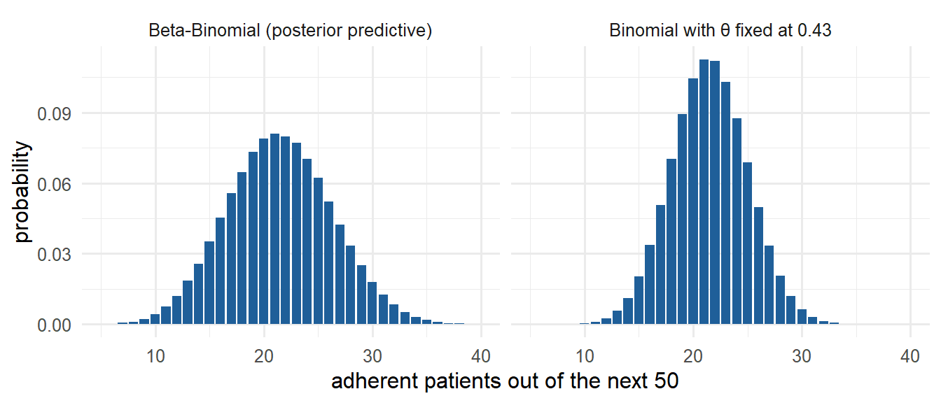
Both have mean \(50 \times 0.43 = 21.5\). The SD is 4.8 for the Beta–Binomial and 3.5 for the plug-in. The chance of at least 25 adherent patients is 0.27 vs 0.20: ignoring parameter uncertainty makes you overconfident, in the tails especially.
The mean of the predictive is just \(\tilde n \times E[\theta \mid y]\), which is why the posterior mean of \(\theta\) is also the predictive probability that one new patient adheres.
2.10 Counts: the Gamma–Poisson model
Counts with exposure \(E\) (patient-days, person-years): \(y \sim \text{Poisson}(E\lambda)\). With a \(\text{Gamma}(\alpha, \beta)\) prior (shape \(\alpha\), rate \(\beta\); mean \(\alpha/\beta\)):
\[\lambda \mid y \sim \text{Gamma}(\alpha + y,\; \beta + E).\]
Add the count to the shape and the exposure to the rate. The prior behaves like \(\alpha\) events in \(\beta\) units of exposure.
Worked example: hospital-acquired infections. Rate \(\lambda\) per 1,000 patient-days. Similar wards have rates of roughly 1 to 9, around 4: prior Gamma(4, 1) (mean 4, 95% interval 1.1–8.8). A ward records 3 infections in 2,500 patient-days (\(E = 2.5\)), observed rate 1.2.
| Distribution | Mean | 95% interval | \(P(\lambda > 3)\) | |
|---|---|---|---|---|
| Prior | Gamma(4, 1) | 4.0 | 1.1–8.8 | |
| After 2,500 patient-days | Gamma(7, 3.5) | 2.0 | 0.8–3.7 | 0.10 |
| After 25,000 patient-days, 30 infections | Gamma(34, 26) | 1.3 | 0.9–1.8 | < 0.001 |
Little exposure: strong shrinkage towards the prior. Ten times the exposure at the same observed rate: the data dominate.
Posterior predictive for the count in the next \(\tilde E\) units: a negative binomial distribution, a Poisson whose rate is itself uncertain (a Gamma mixture of Poissons). It is wider than a Poisson with the same mean. For the next 1,000 patient-days: mean 2.0, \(P(\tilde y \geq 5) = 0.075\) vs 0.053 for a Poisson(2). The same idea gives the negative binomial as a model for overdispersed counts in regression.
2.11 Unknown mean and variance
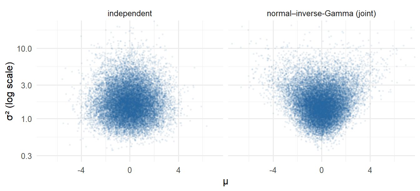
With both \(\mu\) and \(\sigma^2\) unknown you cannot multiply the two one-parameter conjugate priors: the posterior of \(\mu\) depends on \(\sigma\) and vice versa. They have a joint posterior, and the marginal posterior of \(\mu\) means integrating over \(\sigma\):
\[p(\mu \mid y) = \int p(\mu, \sigma \mid y)\, d\sigma.\]
- The joint conjugate prior is the normal–inverse-Gamma: \(\sigma^2 \sim \text{Inv-Gamma}\) and \(\mu \mid \sigma^2 \sim N(\mu_0, \sigma^2/\kappa_0)\). The prior for \(\mu\) is wider when \(\sigma^2\) is large: a funnel shape.
- With the reference prior \(p(\mu, \sigma^2) \propto 1/\sigma^2\) you get \(\dfrac{\mu - \bar y}{s/\sqrt n} \Bigm| y \sim t_{n-1}\): the classical t-interval, with a Bayesian reading. The t distribution appears because the uncertainty about σ has been integrated out.
2.12 Linear models and the limits of conjugacy
The linear model \(y_i \sim N(\alpha + \beta_1 x_{i1} + \dots + \beta_p x_{ip}, \sigma^2)\) needs priors for \(\alpha\), each \(\beta_j\) and \(\sigma\) (not for the \(\mu_i\), which are functions of the parameters). Notes on the joint posterior:
- It is correlated: the intercept correlates with the slopes unless predictors are centred, and non-orthogonal designs correlate the slopes.
- With flat priors on the coefficients and \(1/\sigma^2\) on the variance you recover OLS and its t and \(\chi^2\) results.
- Informative priors make impossible OLS problems possible: with \(p + 1 \geq n\) or collinear predictors, OLS has no unique solution, but a proper prior regularises the problem (ridge regression is the classical analogue). The answer then depends strongly on the prior.
Where conjugacy ends. No conjugate prior exists for Student-t data (robust to outliers), for censored or left-truncated data (values below a detection limit), for logistic regression, or for most multi-parameter models. Grids fail beyond a few parameters. Module 3 solves this with MCMC.
When to use conjugate analysis
- Single-parameter problems where the prior can be stated as a mean and a spread: proportions (Beta), rates (Gamma), means with known variance (normal).
- Quick sanity checks and back-of-the-envelope updates, including checking MCMC output against an exact answer.
- Explaining a Bayesian analysis to collaborators: “the prior is worth 20 patients”.
- Sequential monitoring, where the posterior after each batch becomes the next prior.
Limitations
- Only a short list of likelihood–prior pairs is conjugate. Choosing a prior family because it is conjugate is convenience, not knowledge; with enough data this rarely matters, with little data it can.
- Several parameters with dependence need joint priors that are hard to specify and interpret.
- Truncation, censoring, heavy tails and hierarchical structure all leave the conjugate world.
Part B · Practice in the browser
NoteInteractive R
Cells marked Run Code run R in your browser. The first run on a page takes a few seconds while R loads.
Exercise 1 · Beta–Binomial updating, three panels side by side.
- Make the prior weaker (
prior_sd <- 0.2). How many patients is it worth now, and where does the posterior mean land? - Keep
prior_sd <- 0.1and multiply the data by 10 (90 of 300). What happens to the prior’s influence? - What happens if you ask for
prior_sd <- 0.5? Look ataandband explain.
TipModel answer
- With SD 0.2: a + b = 0.24/0.04 − 1 = 5, so a = 3, b = 2, worth 3 patients. Posterior Beta(12, 23), mean ≈ 0.34, close to the data.
- The posterior mean moves to about 0.32; the 23 “prior patients” are small compared with 300.
- a + b = 0.24/0.25 − 1 < 0, so a and b are negative: no Beta distribution has mean 0.6 and SD 0.5. The largest possible SD for a Beta with mean m is below \(\sqrt{m(1-m)}\) ≈ 0.49, and a moment-matched prior needs a much smaller SD than that to be sensible.
Exercise 2 · Grid approximation vs the exact posterior. The Module 1 recipe on a continuous parameter.
- Try
n_grid <- 10andn_grid <- 1000. How many grid points do you need for the mean to be right to three decimals? - With two parameters and 1,000 points each, how many evaluations does a grid need? With 10 parameters? (This is Module 3’s “curse of dimensionality”.)
TipModel answer
- Already at 100 points the mean agrees to about three decimals; 10 points are visibly coarse. The shape needs more points than the mean.
- 1,000² = one million for two parameters; 1,000¹⁰ = 10³⁰ for ten. Impossible, which is why grids stop at two or three parameters.
Exercise 3 · Normal–normal: how much does the prior pull?
- Add two readings of 47. Check that you get the same answer as the sequential update in Section 2.5.
- With a single reading of 50, what is \(P(\mu > 48)\)? Would you diagnose on one reading?
TipModel answer
readings <- c(52, 48, 47, 47)gives mean 48.0, SD 1.94, as in the table.- Posterior mean ≈ 48.0, SD ≈ 3.6, P(μ > 48) ≈ 0.50: a coin flip. Guidelines require a repeat test, and the posterior shows why.
Why-questions
NoteWhy does the posterior variance always shrink in the normal model, even when data and prior disagree?
Precisions add, and the data precision \(n/\sigma^2\) does not depend on where the data lie. In the Beta–Binomial model this is only approximately true: data near 0.5 can widen the posterior compared with a prior near 0 or 1, because the binomial variance \(\theta(1-\theta)\) depends on the value.
NoteWhy is shrinkage not “bias we should avoid”?
Shrinking towards the prior introduces bias for any individual whose true value is far from the prior mean, but it reduces variance. When many estimates are made (patients, hospitals, genes) the total error is usually smaller. This bias–variance trade-off is the core of Module 5.
NoteWhy is the t distribution a Bayesian result too?
It is the marginal posterior of μ after averaging over the uncertainty about σ. A normal distribution with σ plugged in would ignore that uncertainty and be too narrow, the same lesson as the plug-in predictive in Section 2.9.
Spaced review: Module 1
Note1. What are the two conditions on prior and likelihood for a posterior to exist?
The likelihood must be defined wherever the prior is positive, and some values with positive prior must give the observed data positive probability. (1.4)
Note2. How do you get a 95% interval for exp(θ) from draws of θ?
Exponentiate every draw and take the 2.5th and 97.5th percentiles, or equivalently exponentiate the interval endpoints. Do not exponentiate the mean. (1.5)