Module 4 — Model Checks, Comparisons and Stacking
Convergence is not fit · posterior predictive checks · test statistics and p-values · KL divergence and elpd · AIC, DIC, WAIC, LOO · comparing models · stacking · the estimand from draws
After Module 3 you can fit a model and show that the MCMC converged. That only means you have an accurate picture of the posterior under the model you assumed. A badly wrong model converges just as happily as a good one. Module 4 asks the next questions: Is this model any good? Where does it fall short? Would another model do better?
The first tool is the posterior predictive check (PPC). Because Bayesian models are generative, you can simulate “replicated” datasets from the fitted model and compare them with the data you actually observed. If the replications systematically miss a feature you care about (the tails, the share of zeros, the pattern across subgroups), the model needs work.
The second tool estimates out-of-sample predictive performance. The ideal measure is the expected log predictive density for new data (elpd), rooted in the Kullback–Leibler divergence. AIC, DIC, WAIC and leave-one-out cross-validation (LOO) are increasingly good estimates of it. brms reports LOO with a standard error, so you can see whether a difference between models is larger than its uncertainty.
The third idea is stacking: rather than picking one model, average the predictive distributions of several, with weights chosen for predictive performance. The module ends by computing the actual target of inference, often a non-linear function of parameters, from the draws.
NoteSources, reading and seminar
Course notes: Module 4 “Model checks, comparisons and stacking” (pp. 163–216). Reading deadline: Seminar 4, Monday 28 September 2026 (topic: PPC diagnostics, stacking).
Optional: McElreath, Statistical Rethinking, chapter 7 (overfitting, information criteria, LOO). Gabry et al. (2019), “Visualization in Bayesian workflow”, JRSS A, the source for pp_check() graphics. Vehtari, Gelman and Gabry (2017), “Practical Bayesian model evaluation using leave-one-out cross-validation and WAIC”, Statistics and Computing.
Examples on this page (length of hospital stay, sodium readings with faulty values, flu vaccination by age) are written for this app. The course notes’ own example (school meals and numeracy) is in the notes.
TipBefore you start: three things you need
Posterior predictive distribution (1.6): draw θ from the posterior, then simulate data from \(p(y \mid \theta)\). One such simulated dataset of the same size as your data is a replication \(y^\text{rep}\).
Log-likelihood and deviance. Deviance = −2 × log-likelihood. Higher log-likelihood (lower deviance) means the model gives the data more probability. Adding parameters never lowers the in-sample fit of nested models, which is why complexity must be penalised.
Overfitting. A model tuned too closely to one sample fits that sample well and new data badly. In-sample fit is optimistic; out-of-sample fit is what matters for prediction.
Part A · Concepts
4.1 Convergence is not fit
Two separate questions:
| Question | Tool | Module |
|---|---|---|
| Does my MCMC sample represent the posterior of this model? | Trace plots, R-hat, ESS | 3 |
| Is this model a reasonable description of the data, for my purpose? | Posterior predictive checks, LOO | 4 |
Fit a normal model to data from a heavy-tailed distribution and the chains converge perfectly: R-hat 1.00, thousands of effective draws. Convergence is a property of the algorithm; fit is a property of the model. Check convergence first (otherwise the checks of fit use a wrong posterior), then check fit before interpreting estimates.
WarningCommon confusion: “no warnings from brms, so the model is fine”
brms warns about sampling problems (divergences, R-hat, ESS). It never warns that the likelihood is wrong, that an important predictor is missing, or that the prior is absurd. Those need posterior (and prior) predictive checks and subject-matter thinking.
4.2 Graphical posterior predictive checks
- For many posterior draws \(\theta^{(s)}\), simulate a replicated dataset \(y^{\text{rep}(s)}\) of the same size and with the same covariates as the observed data.
- Compare the replications with the observed \(y\), graphically or through a statistic.
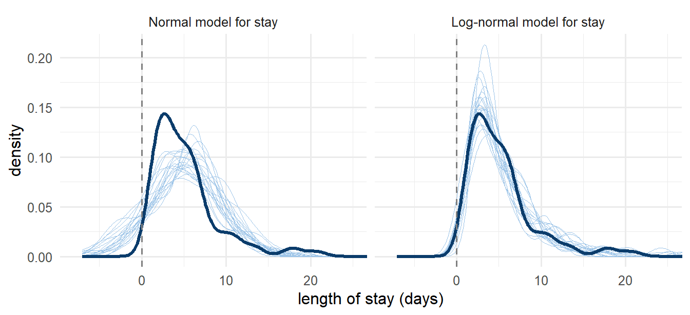
In brms: pp_check(fit) overlays the density of the observed outcome (dark line) on densities of, by default, 10 replications (light lines). ndraws = 50 shows more.
Each replication differs from the others, so no replication will match the data exactly. The question is whether the observed data look like one more replication. On the left, they do not: the observed distribution is skewed, has no negative values and peaks earlier than any replication.
Other useful graphical checks (all pp_check(fit, type = ...)):
type = |
Shows | Good for |
|---|---|---|
"dens_overlay" (default) |
densities of \(y\) and replications | continuous outcomes |
"hist", "ecdf_overlay" |
histograms, cumulative distributions | tails, discreteness |
"stat", "stat_2d" |
a statistic of \(y\) vs its replication distribution | any outcome, incl. binary |
"stat_grouped" |
the statistic within each level of a grouping variable | subgroups, clusters (the variable must be in the model; otherwise use bayesplot::ppc_stat_grouped(), Task 4.2) |
"intervals", "scatter_avg" |
predictive intervals vs observed per observation | outliers, regression fit |
"bars" |
counts per category | ordinal and count outcomes |
4.3 Test statistics and posterior predictive p-values
For a binary outcome, a density plot of zeros and ones says little. Choose a test statistic \(T(y)\) instead: the proportion of ones, the mean in a subgroup, the maximum, the share of zeros, a correlation between repeated measurements. Compute it for the data and for every replication:
\[p_\text{B} = P\big(T(y^\text{rep}) \geq T(y) \mid y\big) \approx \frac{1}{S}\sum_s I\big(T(y^{\text{rep}(s)}) \geq T(y)\big).\]
- A value near 0.5 means the observed statistic sits in the middle of the replications: the model reproduces this feature.
- Near 0 or 1 means the observed value is in a tail: the model misses this feature. The notes suggest treating values below about 0.11 or above 0.89 as a reason to extend the model (the threshold depends on how important the feature is).
- Choose statistics that the model does not fit directly. A model with an intercept will always reproduce the overall mean, so checking the mean is weak. Check what the model does not explicitly fit: tails, subgroups, variables left out of the model, the dependence between repeated measurements.
The overall proportion of ones
The proportion of ones within each region
The mean of the replicated proportion of ones
The number of observations in each replication
The intercept makes the model reproduce the overall proportion almost by construction. A grouping variable that is not in the model (region) is where systematic misfit can show up. The last two options are not checks of fit at all.
WarningCommon confusion: PPCs and multiple testing
Posterior predictive checks are not inferences about parameters or predictions of new data: they are diagnostics, like trace plots. The notes say there is no need to correct for multiple testing. Check as many features as are relevant, then act: extend the model, or report the limitation.
4.4 Choosing checks for your question
Which features matter depends on the research question. Some starting points:
| Data structure | Useful checks |
|---|---|
| Continuous outcome | density overlay; skewness; min and max; share of extreme values |
| Binary outcome | proportion of ones overall and by subgroup (stat_grouped), including groups not in the model |
| Counts | share of zeros; variance vs mean (overdispersion); max |
| Clustered or repeated measures | cluster means (stat_grouped by cluster); SD of cluster means; correlation between time points; scatter of \(y_{i2}\) against \(y_{i1}\), observed vs replicated |
| Items in a questionnaire | item-specific means; log odds ratios between pairs of items |
A failed check points to a specific extension: heavier tails (Student-t), a transformation, a quadratic term or spline, an interaction, a random effect, an overdispersion parameter.
4.5 Robust likelihoods: normal or Student-t?
When a few values are wildly off (transcription errors, faulty samples, a minority of unusual patients), a normal likelihood lets them inflate \(\sigma\) and pull the mean. A Student-t likelihood has heavier tails, so outliers are less “surprising” and have less leverage. In brms: family = student(), with the degrees of freedom \(\nu\) estimated (default prior gamma(2, 0.1)) or fixed via bf(y ~ 1, nu = 4).
- Small \(\nu\) (3–5): heavy tails. Large \(\nu\) (> 30): practically normal.
- The Student-t is not the true model for contaminated data (a mixture of good and bad readings), but it is usually less wrong than the normal. Compare them with PPCs and LOO (Task 4.1).
- \(\sigma\) in a Student-t model is a scale, not the SD: \(\text{SD} = \sigma\sqrt{\nu/(\nu-2)}\) for \(\nu > 2\).
4.6 Out-of-sample performance: KL divergence and elpd
The objective way to judge a model is how well it predicts new data. The notes build the ideal measure from the Kullback–Leibler divergence between the true distribution of new data \(g\) and the model’s predictive distribution \(f\):
\[D_\text{KL}(g \,\|\, f) = \int g(\tilde y) \log\frac{g(\tilde y)}{f(\tilde y)}\,d\tilde y \;\geq 0, \qquad = 0 \text{ only if } f = g.\]
- It is asymmetric: \(D_\text{KL}(g\|f) \neq D_\text{KL}(f\|g)\). A too-narrow prediction that misses where data actually land is punished more than a too-wide one (“the expected surprise” when reality turns out to be \(g\)).
- When comparing models, \(\int g \log g\) is the same constant for all of them, so only \(E_g[\log f(\tilde y)]\) matters. Summed over observations this is the expected log pointwise predictive density:
\[\text{elpd} = \sum_{i=1}^n E_{g_i}\big[\log p(\tilde y_i \mid y)\big].\]
Higher elpd = better predictions. We never know \(g\), so every method below is an estimate of elpd.
4.7 AIC, DIC and WAIC
All three take the in-sample fit and subtract a penalty for complexity to correct its optimism. On the deviance scale: criterion = −2 × (estimated elpd); lower is better.
| Criterion | In-sample fit uses… | Penalty | Notes |
|---|---|---|---|
| AIC | log-likelihood at the MAP/MLE (one point) | \(k\) = number of parameters | ignores posterior uncertainty; assumes a roughly normal posterior |
| DIC | average deviance over posterior draws | posterior variance of the deviance / 2 (one version) | uses the posterior, still assumes near-normality |
| WAIC | \(\text{lppd} = \sum_i \log\Big(\frac1S\sum_s p(y_i \mid \theta^{(s)})\Big)\) | \(p_\text{WAIC} = \sum_i \text{var}_s\big(\log p(y_i \mid \theta^{(s)})\big)\) | pointwise, fully Bayesian, no normality assumption |
\(\text{elpd}_\text{WAIC} = \text{lppd} - p_\text{WAIC}\), and \(\text{WAIC} = -2\,\text{elpd}_\text{WAIC}\). The penalty \(p_\text{WAIC}\) is an “effective number of parameters”: with strong priors or hierarchical shrinkage it is smaller than the raw parameter count.
Because WAIC (and LOO) are sums over observations, you get a standard error from the pointwise terms, and a paired standard error for the difference between two models (Section 4.9).
4.8 Leave-one-out cross-validation
Cross-validation estimates elpd directly: fit on part of the data, evaluate the log predictive density on the held-out part. No penalty is needed, because the test data were not used for fitting.
- k-fold CV: split into \(k\) folds, fit \(k\) times. Each fit uses a fraction \((k-1)/k\) of the data.
- LOO-CV: \(k = n\). Refitting \(n\) times is expensive, but PSIS-LOO (Pareto-smoothed importance sampling) approximates it from a single fit:
loo(fit)in brms. - Pareto \(\hat k\) diagnostics. Each observation gets a \(\hat k\). Values below 0.7 are fine. Above 0.7, that observation is highly influential and the approximation is unreliable for it: use
loo(fit, moment_match = TRUE)(the model must be fitted withsave_pars = save_pars(all = TRUE)),loo(fit, reloo = TRUE), orkfold(fit, K = 10).
What does “leave one out” mean for your data? LOO answers “how well do I predict a new observation from a group I have already seen?” To predict a new group (a new hospital, region or country), leave out whole groups: kfold(fit, folds = "grouped", group = "hospital", K = 10). For time series, predict the future from the past. The notes recommend LOO-PSIS or k-fold over WAIC; LOO also gives the \(\hat k\) warnings that WAIC lacks.
4.9 Comparing models
loo_compare(loo(fit_a), loo(fit_b))
#>        elpd_diff se_diff
#> fit_b    0.0       0.0
#> fit_a -12.3 4.1- The best model is on the top row, with
elpd_diff = 0. Other rows show how much worse they are, with the standard error of the paired difference. - Rules of thumb (notes, based on Stan’s LOO FAQ): trust a difference only if \(|\text{elpd\_diff}| > 4\) and it is larger than about 2 ×
se_diff. Above: difference −12.3 with SE 4.1 → about 3 SE, so a real advantage forfit_b. - Works for non-nested models (logit vs probit, normal vs Student-t) and different likelihoods, as long as they predict the same outcome on the same scale. A model for log(y) must include the Jacobian to be compared with a model for \(y\) (brms handles this when you model
lognormal()rather thanlog(y)). - The comparison includes the prior: a model is “model + prior”.
B predicts clearly better, so choose B
No clear difference: consider both, or the simpler one
A predicts better, because its elpd_diff is negative
The standard error is too large, so LOO has failed
|−2.1| < 4 and about 1.2 SE: within the noise of the estimate. Report both, check whether they lead to the same conclusions, or stack them. A negative elpd_diff means worse than the top model.
WarningCommon confusion: model comparison as variable selection
Choosing variables by repeated model comparison is a data-driven search with the same multiple-testing problems as stepwise selection, and the chosen model’s intervals are too narrow. Use comparison to learn which features predict and which patterns a model misses; choose adjustment variables from subject-matter knowledge (confounders) instead.
4.10 Stacking and Bayesian model averaging
If several models predict reasonably well, a weighted average of their predictive distributions often predicts better than any single one, without fitting a new model:
\[p(\tilde y \mid y, \text{stack}) = \sum_j w_j\, p(\tilde y \mid y, \text{model}_j), \qquad w_j \geq 0,\; \sum_j w_j = 1.\]
- WAIC or LOO weights (“pseudo-BMA”, as in the notes): \(w_j = \dfrac{\exp(-\tfrac12 \text{WAIC}_j)}{\sum_k \exp(-\tfrac12 \text{WAIC}_k)}\). A model a few WAIC units worse gets a small weight; one much better gets nearly all.
- Stacking weights: choose \(w\) to maximise the LOO predictive density of the mixture. Models that are good in different regions of the data both get weight.
- In brms:
loo_model_weights(list(a = loo_a, b = loo_b), method = "stacking")or"pseudobma";pp_average(fit_a, fit_b)gives the averaged predictions. - Sampling from the stack: take \(w_j \times S\) draws from model \(j\)’s posterior predictive, then combine.
Why it helps. Two models that err in opposite directions in some region cancel part of each other’s error. If one model is better everywhere, it gets (nearly) all the weight and stacking changes nothing.
Caution. Stacking is for prediction. Averaging a parameter across models is often meaningless, because “the coefficient of x” means something different when the other covariates differ.
4.11 The estimand, computed from the draws
Once a model checks out, compute the quantity that answers your research question, which is rarely a raw coefficient:
- a risk difference or risk ratio at chosen covariate values (from
posterior_epred), rather than a log odds ratio; - a ratio of two effects (“the intervention is worth 0.6 years of learning” in the notes’ school meals example is
b_meals / b_wave); - a probability of a clinically relevant effect, \(P(\text{effect} > \delta \mid y)\);
- ranks or the probability of being best (Module 5).
Recipe: draws → compute the estimand in every draw → summarise (median, 95% interval, probabilities). Non-linear functions need no delta method: uncertainty propagates automatically.
When to use which check
- Always: convergence diagnostics, then at least one graphical PPC and one or two test statistics targeted at your question.
- Choosing between plausible models (likelihoods, links, functional forms, random-effect structures): LOO with
loo_compare, plus PPCs showing where they differ. - Pure prediction with several decent models: stacking.
Limitations
- PPCs use the data twice (to fit and to check), so they are conservative: they find gross misfit more easily than subtle misfit. p-values near 0.5 do not prove the model right.
- LOO estimates prediction for data like yours. It cannot detect confounding, and a model with better predictions is not necessarily the right causal model.
- LOO is unreliable with many high Pareto \(\hat k\) values (small clusters, very flexible models); use k-fold CV then.
- Information criteria compare models on the same outcome. They cannot compare models fitted to different datasets or different transformations without adjustment.
Part B · Practice
In the browser: a posterior predictive check and WAIC by hand
NoteInteractive R
Runs in your browser. A normal model with unknown mean and SD and the reference prior has an exact posterior (2.11), so no MCMC is needed.
- Which statistics does model A fail? What share of model A’s replicated stays are negative (
mean(yrep_A < 0))? - Invent a statistic that model B might fail, for example the share of stays longer than 14 days. Check it.
TipModel answer
- Model A fails the minimum (p ≈ 0.001: replicated minima are almost always below the observed 1.1 days, usually negative) and skewness (p ≈ 0: the data are right-skewed, the normal is symmetric). The maximum is borderline (p ≈ 0.07). About 7% of replicated stays are negative, which is impossible. Model B’s p-values are all between 0.3 and 0.8.
ppp(yrep_B, function(y) mean(y > 14))is around 0.5. Model B passes, as it should, since these data were simulated from a log-normal. With real data, look for features that matter clinically: the share of very long stays drives bed planning.
- Interpret the difference using the rules of thumb from Section 4.9.
- Why are the weights so extreme?
- Why would comparing
dnorm(log(y), ...)for model B withdnorm(y, ...)for model A be wrong?
TipModel answer
- Model B’s elpd is about 20 higher, with an SE of the difference of about 5: more than 4 and about 4 SE. A clear predictive advantage for the log-normal.
- A WAIC difference of 40 means a weight ratio of \(e^{20}\): essentially all weight goes to B. Pseudo-BMA weights are extreme whenever one model is clearly better. Stacking behaves similarly here, since B is better everywhere.
- They would be densities for different variables (days vs log-days). A density for log(y) must be divided by y (the Jacobian) to become a density for y;
dlnormdoes exactly that. Otherwise the comparison mixes units.
In RStudio: brms tasks
ImportantHow the RStudio tasks work
Each task simulates its own data. Try first, then open the solution. The solutions were run with brms 2.23; your numbers will differ slightly. Download all Module 4 tasks: module4-tasks.R.
Task 4.1 · Normal or Student-t for sodium readings with some faulty values
set.seed(520)
bad_reading <- rbinom(300, size = 1, prob = 0.05)
sodium <- data.frame(value = ifelse(bad_reading == 1,
                                    rnorm(300, mean = 140, sd = 15),
rnorm(300, mean = 140, sd = 3)))- Fit
value ~ 1withfamily = gaussian()and withfamily = student()(priors: Interceptnormal(140, 10), sigmaexponential(0.2), nugamma(2, 0.1)). Do both converge? - Compare
pp_check(fit, ndraws = 50)for the two models. - Define
share_near <- function(y) mean(abs(y - 140) < 3)andshare_extreme <- function(y) mean(abs(y - 140) > 15). Usepp_check(fit, type = "stat", stat = "share_near")and compute the posterior predictive p-values by hand. - Compare the models with
loo_compare().
TipSolution
fit_normal <- brm(value ~ 1, family = gaussian(),
                  prior = c(prior(normal(140, 10), class = "Intercept"),
                            prior(exponential(0.2), class = "sigma")),
                  data = sodium, chains = 4, iter = 2000, seed = 520, refresh = 0)
fit_student <- brm(value ~ 1, family = student(),
                   prior = c(prior(normal(140, 10), class = "Intercept"),
                             prior(exponential(0.2), class = "sigma"),
                             prior(gamma(2, 0.1), class = "nu")),
                   data = sodium, chains = 4, iter = 2000, seed = 520, refresh = 0)
pp_check(fit_normal, ndraws = 50) + xlim(110, 170)
pp_check(fit_student, ndraws = 50) + xlim(110, 170)

yrep_normal  <- posterior_predict(fit_normal)
yrep_student <- posterior_predict(fit_student)
mean(apply(yrep_normal, 1, share_near) >= share_near(sodium$value))
mean(apply(yrep_student, 1, share_near) >= share_near(sodium$value))
# ... and the same for share_extreme
loo_compare(loo(fit_normal), loo(fit_student))
What we got: both converge (Rhat 1.00, ESS > 2,000). Normal: mean 140.08, sigma 4.79, inflated by the faulty readings (the good readings have SD 3). Student-t: mean 139.79, sigma 2.96, nu 3.7 (heavy tails).
Test statistics. Observed: 59.7% of readings lie within 3 mmol/L of 140, and 1.7% lie more than 15 away.
share_near |
share_extreme |
|
|---|---|---|
| Normal model, p-value | 0.0003 | 0.0003 |
| Student-t model, p-value | 0.77 | 0.23 |
The normal model fails both checks: with σ = 4.8 it expects about 47% of readings near 140 (too few) and about 0.2% beyond 15 (too few). It cannot have a sharp peak and heavy tails at the same time. The Student-t passes both. The density overlay shows the same thing: the normal replications are too flat in the middle.
loo_compare: the Student-t model is on top; the normal model has elpd_diff = −55.8 with se_diff = 19.2, about 3 SE. The heavy-tailed model predicts clearly better. All Pareto \(\hat k\) < 0.7.
Task 4.2 · A binary outcome: flu vaccination by age
set.seed(521)
vaccine <- data.frame(age = round(runif(800, min = 20, max = 85)))
true_logodds <- -1.2 + 0.0008 * (vaccine$age - 20)^2       # uptake accelerates with age
vaccine$vaccinated <- rbinom(800, size = 1, prob = plogis(true_logodds))
vaccine$age10 <- (vaccine$age - 50) / 10
vaccine$age_group <- cut(vaccine$age, breaks = c(19, 35, 50, 65, 75, 85))- Fit
vaccinated ~ age10(family = bernoulli(), priorsnormal(0, 1.5)Intercept andnormal(0, 1)b). Checkpp_check(fit, type = "stat", stat = "mean"). Is that a useful check? - Check the share vaccinated within each age group. Where does the model fail? Note:
pp_check(fit, type = "stat_grouped", group = "age_group")stops with “Variable ‘age_group’ could not be found in the data”: brms only accepts grouping variables that are in the model, even withnewdata. Call bayesplot directly instead:bayesplot::ppc_stat_grouped(y = vaccine$vaccinated, yrep = posterior_predict(fit), group = vaccine$age_group, stat = "mean"). - Fit
vaccinated ~ age10 + I(age10^2)and repeat. Compare the two models with LOO.
TipSolution
fit_linear <- brm(vaccinated ~ age10, family = bernoulli(),
                  prior = c(prior(normal(0, 1.5), class = "Intercept"),
                            prior(normal(0, 1), class = "b")),
                  data = vaccine, chains = 4, iter = 2000, seed = 521, refresh = 0)
fit_quadratic <- brm(vaccinated ~ age10 + I(age10^2), family = bernoulli(),
                     prior = c(prior(normal(0, 1.5), class = "Intercept"),
                               prior(normal(0, 1), class = "b")),
                     data = vaccine, chains = 4, iter = 2000, seed = 521, refresh = 0)
pp_check(fit_linear, type = "stat", stat = "mean")

yrep_linear    <- posterior_predict(fit_linear)
yrep_quadratic <- posterior_predict(fit_quadratic)
bayesplot::ppc_stat_grouped(y = vaccine$vaccinated, yrep = yrep_linear,
                            group = vaccine$age_group, stat = "mean")
bayesplot::ppc_stat_grouped(y = vaccine$vaccinated, yrep = yrep_quadratic,
                            group = vaccine$age_group, stat = "mean")
loo_compare(loo(fit_linear), loo(fit_quadratic))
What we got: the overall mean check is useless here. Both models reproduce the overall share almost by construction, and brms itself warns that “mean” is a weak statistic.
Share vaccinated per age group, with the posterior predictive p-value \(P(\text{replicated share} \geq \text{observed})\):
| Age group | Observed | Linear: replicated 5%–95% | p (linear) | p (quadratic) |
|---|---|---|---|---|
| 20–35 | 0.28 | 0.15–0.28 | 0.05 | 0.34 |
| 36–50 | 0.30 | 0.31–0.45 | 0.97 | 0.79 |
| 51–65 | 0.49 | 0.49–0.63 | 0.97 | 0.73 |
| 66–75 | 0.78 | 0.62–0.78 | 0.07 | 0.09 |
| 76–85 | 0.83 | 0.72–0.87 | 0.22 | 0.73 |
The linear model shows a systematic pattern: too low at the youngest and at 66–75, too high in the middle. That is the signature of a curved relationship forced into a straight line on the logit scale. The quadratic model removes the pattern (one group is borderline at 0.09, which is what you expect by chance among five checks).
loo_compare: quadratic on top, linear −4.2 with SE 3.3. Just above 4 but only 1.3 SE: by the rules of thumb, not a clear difference. The PPC detected a systematic misfit that the LOO average hardly registers, because LOO sums over all 800 people and the misfit is modest for each. PPCs target the features you care about; LOO answers a more general question.
Task 4.3 · Stacking weights
Using the two LOO objects from Task 4.2, compute loo_model_weights(..., method = "stacking") and method = "pseudobma". Do the two methods agree? When would they differ?
TipSolution
loo_linear    <- loo(fit_linear)
loo_quadratic <- loo(fit_quadratic)
loo_model_weights(list(linear = loo_linear, quadratic = loo_quadratic), method = "stacking")
loo_model_weights(list(linear = loo_linear, quadratic = loo_quadratic), method = "pseudobma")
What we got: stacking gives the linear model 0.11 and the quadratic 0.89; pseudo-BMA+ gives 0.13 and 0.87. They agree because the quadratic model is better almost everywhere. They would differ if each model predicted better in a different part of the data (say, one better for the young and the other for the old): stacking would then keep both with substantial weight, while pseudo-BMA would still favour the one with the higher total elpd.
Task 4.4 · The estimand: how much more likely is a 70-year-old to be vaccinated than a 40-year-old?
Using the quadratic model, compute the posterior of the risk difference \(P(\text{vaccinated} \mid 70) - P(\text{vaccinated} \mid 40)\) with posterior_epred(). Report the median, a 95% interval and \(P(\text{difference} > 0.3)\).
TipSolution
ages_of_interest <- data.frame(age10 = c((40 - 50) / 10, (70 - 50) / 10))
risk_draws <- posterior_epred(fit_quadratic, newdata = ages_of_interest)   # draws x 2
risk_difference <- risk_draws[, 2] - risk_draws[, 1]
quantile(risk_difference, c(0.025, 0.5, 0.975))
mean(risk_difference > 0.3)
What we got: median risk difference 0.40, 95% credible interval 0.33 to 0.46, and \(P(\text{difference} > 0.3 \mid y) \approx 0.999\). A 70-year-old is about 40 percentage points more likely to be vaccinated than a 40-year-old. That sentence answers the question directly, which a log-odds coefficient for age10 and another for its square do not.
Why-questions
NoteWhy check features the model does not fit directly?
A model reproduces what it was built to reproduce: an intercept guarantees the overall mean, a group term guarantees the group means. Misfit shows up in features that were not built in: tails, subgroups, dependence, variables left out.
NoteWhy does WAIC need a penalty but cross-validation does not?
WAIC evaluates the model on the same data used to fit it, which is optimistic; the penalty corrects for that optimism. Cross-validation evaluates on held-out data, so there is no optimism to correct (only a small pessimism, because each fit uses fewer observations).
NoteWhy is the standard error of an elpd difference smaller than the two separate standard errors suggest?
Both models are evaluated on the same observations, so their pointwise elpd values are strongly correlated. The paired SE uses the variance of the pointwise differences, which removes the shared variation between observations.
Spaced review: Modules 1–3
Note1. What is the difference between posterior_epred and posterior_predict?
epred: draws of the expected outcome (the mean, a probability). predict: draws of a new observation, which adds the outcome’s own randomness. (3.12)
Note2. Your summary shows Rhat 1.00 but 50 divergent transitions. Can you trust it?
Not yet. Divergences mean the sampler may have missed a region of the posterior, so estimates may be biased. Increase adapt_delta, and consider reparameterising or tighter priors. (3.7)
Note3. Why does a Beta(1, 1) prior give credible intervals with roughly nominal coverage?
It adds no information, so the posterior is driven by the likelihood like a classical interval. Priors centred away from the truth under-cover. (2.8)