flowchart TD
  A["genotypes"] --> B["QC"]
  B --> C["GWAS"]
  C --> D["significant SNPs"]
  D --> E["LD between them"]
  E --> F["independent signals"]
Computer exercises: concepts
The ideas behind computer exercises 1 and 2, practised on made-up and simulated data
The two computer exercises turn Lectures 4–6 into a working pipeline. Exercise 1 goes from genotypes to a GWAS and then reduces many significant SNPs to a few independent signals, first with individual-level data and then with published summary statistics. Exercise 2 uses those independent signals as instruments in a Mendelian randomization of LDL-C on coronary artery disease.
This page is not a solution to the exercises. It uses its own made-up tables and simulated data so you can practise the concepts and interpretations: what each QC filter does, how to read association output, how clumping works, how to align alleles between two files, and how to read IVW, MR-Egger and weighted median results. Then do the exercises yourself with the course data.
NoteWhat is and is not on this page
Included: concepts, the logic of each step, interpretation, and practice on invented numbers (two drills generate new problems every time).
Not included: code for the exercise tasks, results from the course data (chromosome 19, GLGC, CAD), or answers to the exercises’ own questions. The theory behind the exercises’ final questions is in the lecture sections linked below.
The workflow
flowchart TD
  A["GWAS summary statistics"] --> C["match variants and alleles"]
  B["external genotype reference"] --> C
  C --> D["LD in the reference"]
  D --> E["independent signals"]
flowchart TD
  A["independent exposure SNPs"] --> B["look up in outcome GWAS"]
  B --> C["align alleles"]
  C --> D["Wald ratios"]
  D --> E["IVW + MR-Egger + weighted median"]
  E --> F["interpretation"]
| Step | Theory in the lectures |
|---|---|
| Allele frequency, MAF, per-allele β | 4.2, 4.4 |
| Summary statistics columns | 4.6 |
| Manhattan plot, 5×10⁻⁸ | 4.7 |
| Lead SNP, locus, r² | 4.8, 5.3 |
| LD clumping | 5.4b |
| LD from summary statistics, reference panels | 5.5, 5.6 |
| MR assumptions, IVW, Egger, weighted median | 6.5, 6.7, 6.8 |
Part A: from genotypes to independent signals
A1. PLINK 2 files and genotype QC
PLINK 2 stores a genotype dataset as three files with the same name:
| File | Contents |
|---|---|
.pgen |
The genotype matrix itself (every individual × every variant), in a compact binary format |
.pvar |
One row per variant: chromosome, position, ID (rsID), reference and alternative allele. .pvar.zst is a compressed version (read with vzs) |
.psam |
One row per sample (individual): IDs, sex and similar |
QC filters and why they are used
| PLINK flag | Keeps | Why |
|---|---|---|
--snps-only just-acgt |
Single-nucleotide variants with plain A/C/G/T alleles | Drops indels and odd allele codes that complicate matching between datasets |
--min-alleles 2 --max-alleles 2 |
Biallelic variants | The additive 0/1/2 model assumes exactly two alleles |
--maf 0.01 |
MAF ≥ 1% | Very rare variants give unstable estimates (A2 below) and are prone to genotyping error |
--geno 0.02 |
Variants with ≥ 98% of genotypes called | A variant that fails in many samples is technically unreliable (per-variant missingness) |
--mind 0.02 |
Individuals with ≥ 98% of genotypes called | A sample with many missing calls suggests poor DNA quality (per-individual missingness) |
The same idea returns in proteomics QC (8.6): check both the features (variants, proteins) and the samples (people).
The MAF filter removed most variants, so the panel is mostly rare
An unusual share of people had many missing genotype calls
Many variants failed to genotype in most of the samples
The array must be multiallelic, since many variants were removed
8% of the individuals (240 of 3,000) failed the per-individual call rate, far more than the few hundred variants removed by –geno would suggest. That points to sample problems (DNA quality, a bad plate or batch) worth investigating before the GWAS. Read your own exercise log the same way: which filter removed most, and does that make sense for this kind of data?
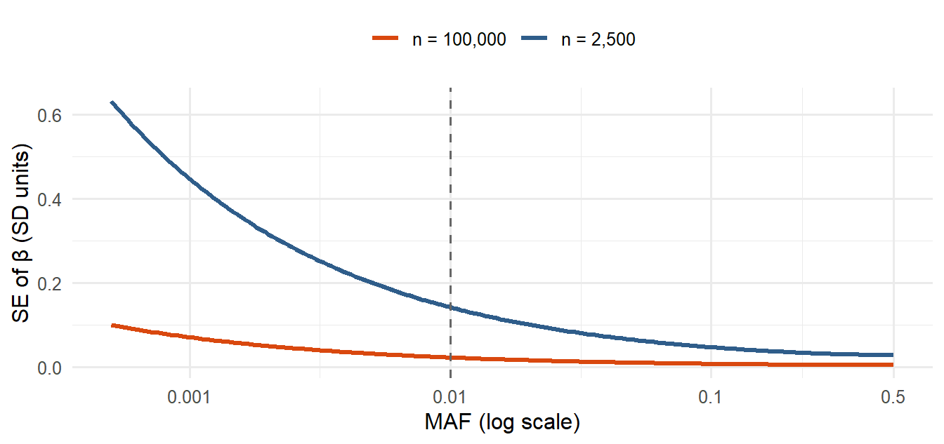
A2. Why rare variants are hard for single-SNP regression
The standard error of the per-allele β shrinks with the number of carriers. For a continuous phenotype with residual SD \(\sigma\) and \(n\) people, approximately
\[\text{SE}(\hat\beta) \approx \frac{\sigma}{\sqrt{2\,n\,\text{MAF}\,(1-\text{MAF})}}\]
because the variance of the 0/1/2 dosage under HWE is \(2\,\text{MAF}(1-\text{MAF})\). With MAF = 0.001 in 2,500 people you expect only about 5 carriers, so β rests on a handful of people: huge SE, low power, and sensitivity to a single genotyping error.
A3. Reading association output
A PLINK --glm linear regression file has one row per variant and test. Invented example:
#CHROM  POS       ID          REF  ALT  A1  TEST  OBS_CT  BETA     SE       T_STAT   P
19      11100000  rs1000001   G    A    A   ADD   2450    -0.312   0.041    -7.61    3.9e-14
19      11100000  rs1000001   G    A    A   AGE   2450     0.021   0.004     5.25    1.6e-07
19 44900000 rs1000002 C T T ADD 2450 0.205 0.035 5.86 5.3e-09| Column | Meaning |
|---|---|
A1 |
The allele β refers to (counted 0/1/2) |
TEST |
ADD = the additive genotype effect; other rows are covariates (hidden with hide-covar) |
OBS_CT |
Number of people in the model |
BETA, SE, T_STAT, P |
Per-A1-allele effect, its standard error, t = β/SE, p-value |
Each G allele lowers the phenotype by 0.312 units
Each A allele lowers the phenotype by 0.312 units
The A allele explains 31.2% of the phenotype variance
Age lowers the phenotype by 0.312 units per year
β is per copy of A1, here A. The AGE row is a covariate. β says nothing about variance explained.
A4. Significant SNP, lead SNP, independent signal
| Term | What it is |
|---|---|
| Significant SNP | Any SNP with p below the threshold (e.g. 5×10⁻⁸). Many can come from one causal variant |
| Lead SNP | The strongest (smallest p) SNP in a region; the representative of a peak |
| Independent signal | What is left after clumping: lead SNPs with r² below the threshold (e.g. < 0.01) to each other |
| Causal SNP | The variant that actually changes biology. It may be a lead SNP, a SNP in LD with it, or not genotyped at all |
Does distance predict LD? Only roughly. LD tends to decay with distance, but recombination hotspots, allele frequencies and population history make the relationship very noisy. Always compute r².
Warning in annotate("label", x = -500, y = 0.12, label = "dashed: r² = 0.01", :
Ignoring unknown parameters: `label.size`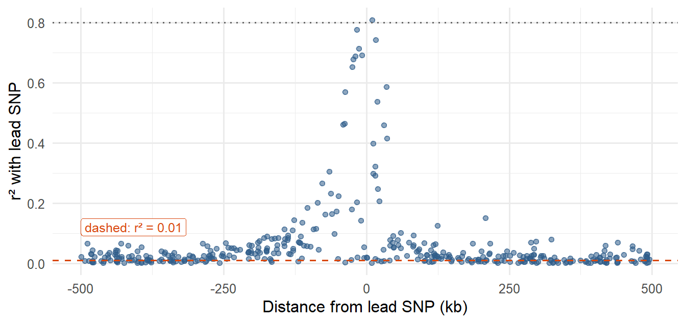
A5. Manual LD clumping
The algorithm used in the exercises:
- Among the remaining significant SNPs, pick the smallest p-value as a lead SNP.
- Compute r² between it and every other remaining significant SNP.
- Remove all SNPs with r² ≥ 0.01 (they are “the same signal”).
- Keep the lead as one signal and repeat from step 1 until nothing is left.
Practise on invented tables. The drill gives a new table each time.
TipCommon mistakes in clumping
- Starting from a SNP that is not the strongest remaining one.
- Comparing with SNPs that have already been removed.
- Using a threshold in the wrong direction (remove r² ≥ 0.01, keep r² < 0.01).
- Concluding that the lead SNPs are causal. They are the strongest statistical signals. A simulated phenotype, where the causal SNPs are known, is exactly the situation where you can check this.
Part B: summary statistics and a reference panel
B1. Why an external reference is needed
Summary statistics have one row per SNP and no individual genotypes, so the correlation between two SNPs (LD) cannot be computed from them. You need a reference panel with individual-level genotypes, e.g. 1000 Genomes, from a population with matching ancestry, because LD patterns differ between populations. → 5.5
Things that go wrong when matching the two:
| Problem | Why it happens | Handling |
|---|---|---|
| SNP missing from the reference | Rare in that population, not in the panel, filtered by QC, or a different ID | Accept the loss, or use a proxy SNP (6.1) |
| Different genome builds | Positions differ between hg19/GRCh37 and hg38/GRCh38 | Match on rsID, which does not depend on the build |
| Different allele coding | Effect allele differs, or the other DNA strand is reported | Align alleles (B2) |
B2. Allele alignment
Before combining two files (GWAS + reference, or exposure + outcome in MR) every SNP must refer to the same effect allele.
| Exposure alleles (effect/other) | Outcome alleles (effect/other) | Case | Action |
|---|---|---|---|
| A / G | A / G | Same | Keep β |
| A / G | G / A | Swapped | Flip the sign of the outcome β (and use 1 − EAF) |
| A / G | T / C | Other strand (complement) | Complement → A/G: keep β |
| A / G | C / T | Other strand and swapped | Complement → G/A: flip the sign |
| A / G | A / C | Incompatible | Exclude |
| A / T or C / G | same letters | Palindromic: the complement is the same pair, so strand is invisible | Use EAF: if clearly far from 0.5, compare EAFs to decide; if close to 0.5, exclude |
They are always multiallelic and fail QC
Their complement is the same allele pair, hiding strand flips
They cannot be tested with the additive model
They never reach genome-wide significance
For A/G you can spot a strand flip because the other strand reads T/C. For A/T the other strand also reads A/T (T/A), so a flip is invisible from the letters. Allele frequencies can resolve it only when the EAF is clearly different from 0.5.
Part C: from independent signals to Mendelian randomization
C1. The MR pipeline in Exercise 2, as concepts
| Step | Why | Theory |
|---|---|---|
| Keep exposure SNPs with p < 5×10⁻⁸ | Relevance: instruments must be strongly associated with the exposure | 6.5 |
| Restrict to SNPs present in the reference panel | LD can only be computed for SNPs that exist there | 5.5 |
| Keep IDs that start with “rs” | Stable identifiers for matching across files and builds | 3.3c |
| LD clumping at r² < 0.01 | Instruments must be independent, or the same signal is counted several times | 5.4b |
| Look up the lead SNPs in the outcome GWAS | Need βoutcome for each instrument; missing SNPs are lost (or replaced by proxies) | 6.1 |
| Align alleles | βexposure and βoutcome must refer to the same allele | B2 above |
| Wald ratio per SNP; IVW, MR-Egger, weighted median | Estimate and check robustness | 6.7, 6.8 |
A common convention is to orient every SNP so that the effect allele raises the exposure (βexposure > 0), flipping both betas when needed. The MR scatter plot then lies in the right half.
C2. Reading an MR analysis: a simulated example
Simulated data, not the course data: 30 independent instruments with a true causal effect of 0.5 (log-odds of the outcome per unit exposure). Four instruments also have a direct effect on the outcome (horizontal pleiotropy).
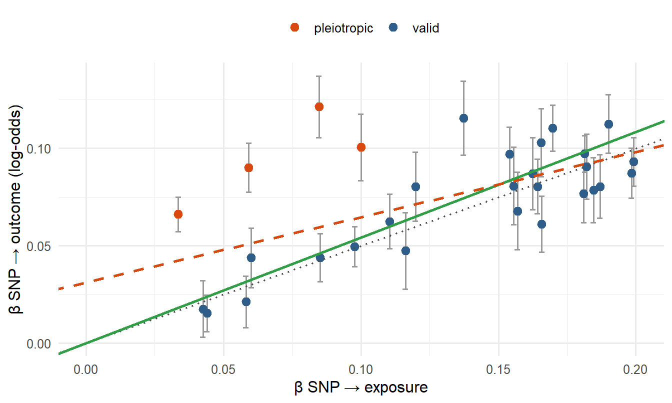
| Method | Estimate | p-value |
|---|---|---|
| IVW | 0.543 | 2.3e-15 |
| MR-Egger (slope) | 0.335 | 8.4e-05 |
| MR-Egger (intercept) | 0.031 | 0.004 |
| Weighted median | 0.505 | n/a |
How to read it
- IVW uses all instruments and assumes they are all valid. With positive pleiotropy in a few SNPs it is pulled upward.
- Weighted median is robust as long as at least ~50% of the weight comes from valid instruments. Here it should be closer to 0.5.
- MR-Egger’s intercept estimates the average pleiotropic effect. Here it is clearly non-zero, signalling directional pleiotropy. The Egger slope is meant to be the pleiotropy-adjusted estimate, but in this simulation it lands well below the truth: with only four pleiotropic SNPs among 30, the free intercept over-corrects. Egger is imprecise and relies on its own assumption (InSIDE), so treat its slope as a sensitivity check, not the answer.
- Agreement in direction across the three methods supports a causal effect; the size of the estimates should be interpreted with the exposure unit in mind (6.9).
Consistent evidence of a positive effect, no sign of directional pleiotropy
The Egger intercept shows strong pleiotropy, so IVW is invalid
The methods disagree in direction, so no conclusion is possible
The effect is negative, since Egger’s slope is smaller than IVW
All three estimates are positive and similar, and the Egger intercept is close to zero and non-significant. That is the triangulation pattern that strengthens a causal interpretation. The Egger p-value is larger simply because Egger is less precise.
A strong and robust causal effect, since IVW is the main method
IVW is probably driven by pleiotropic instruments; be cautious
The weighted median is wrong because its p-value is not significant
Egger’s intercept confirms that the instruments are all valid
The robust method (weighted median) finds almost nothing, and the Egger intercept indicates directional pleiotropy. IVW, which assumes all instruments are valid, is then likely biased. Look for outlying instruments and do not claim causality from IVW alone.
Nothing, because IVW only uses βexposure
Those five points land on the wrong side of the line
All points move closer to the origin by the same amount
The Wald ratios of those five SNPs become exactly zero
A swapped allele gives the outcome β the wrong sign, so those SNPs point in the opposite direction from the rest. They pull IVW toward zero and can create a spurious Egger intercept. This is why allele alignment comes before any MR estimate.
Concept questions to prepare with
The exercises end with concept questions. The theory behind them is in these sections; try explaining each in your own words before you look:
| Concept | Where |
|---|---|
| One signal gives many significant SNPs | 4.8, 5.3 |
| Significant SNP vs lead SNP vs independent signal | A4 above, 4.10 |
| Lead SNP vs causal SNP | 5.3, 5.4 |
| LD cannot come from summary statistics alone | 5.5 |
| Ancestry of the reference panel | 5.4b, 5.5 |
| Allele compatibility | B2 above, 5.6 |
| Clumping before MR | 5.4b, 6.5 |