Lecture 9 — Two-sample MR and polygenic risk scores

One- vs two-sample MR · summary data · selecting instruments and the F-statistic · harmonisation · Wald ratio and IVW · interpreting units · practical pitfalls · PRS vs MR · the PRS formula · discovery and target data · clumping + thresholding and shrinkage · evaluating a PRS · worked paper: remnants vs LDL in UK Biobank

Lecture 6 introduced Mendelian randomization (MR) as if one study measured everything: the genotypes, the exposure and the outcome in the same people. In practice that is rare. The large GWAS of LDL cholesterol and the large GWAS of coronary artery disease were done in different cohorts, and both publish only summary statistics (β, SE, P per SNP). Two-sample MR combines those two sets of summary statistics: the SNP → exposure effects from one GWAS and the SNP → outcome effects from another. No individual-level data is needed, which is why it has become the standard way MR is done.

The price is careful bookkeeping. The same SNP must be found in both files, its alleles must refer to the same strand and the same effect allele (harmonisation), and the two GWAS must describe comparable populations. The three MR assumptions do not go away.

The second half turns from causation to prediction. The same GWAS results can be used to add up a person’s many small genetic effects into a polygenic risk score (PRS). MR asks does X cause Y?; a PRS asks who is at higher risk? The lecture’s arc is association → causal inference → prediction.

This page covers what makes MR “two-sample”, the data it needs, the workflow (select instruments, find them in the outcome GWAS, harmonise, estimate, sensitivity analyses, interpret), the practical pitfalls, and then PRS: the formula, the data it needs, how SNPs are chosen, and how a PRS is interpreted and evaluated. It ends with a real study from Gothenburg, given as extra material (Section 9.14), that uses multivariable MR and polygenic scores to ask whether remnant particles are more harmful than LDL particles.

Sources and session

Slides: “Lecture 9 PRS and 2sample MR.pdf” (27 slides). The title slide also mentions a course summary, but the PDF contains no summary slides.

Reading material (course reading; marked in the text so you can tell it apart from the slides):

(tutorial): Choi, Mak & O’Reilly (2020), “Tutorial: a guide to performing polygenic risk score analyses”, Nature Protocols 15:2759–2772. The reading material for this lecture.
(GWAS primer): Uffelmann et al. (2021), “Genome-wide association studies”, Nature Reviews Methods Primers 1:59. The course’s GWAS paper (Lecture 4); its sections “Risk prediction”, the winner’s curse box and the Mendelian randomization paragraph are relevant here.
(course book): Gomez-Verjan & Rivero-Segura (eds.), Principles of Genetics and Molecular Epidemiology (Springer 2022), chapter 12 “Bioinformatics and Genomics for Epidemiologists” (Bello-Chavolla et al.), section “Polygenic Risk Scores”, pp. 138–139.

Extra material (beyond the required reading):

(extra material): Björnson et al. (2023), “Triglyceride-rich lipoprotein remnants, low-density lipoproteins, and risk of coronary heart disease: a UK Biobank study”, European Heart Journal 44:4186–4195. Used as the worked example in Section 9.14.

Rough plan: Week 5 (29 September). Connects directly to computer exercise 2, which the slides reference (“As in exercise 2. We combine summary data from two sources”).

Before you start: three things from Lectures 4–6

Summary statistics (4.6): one row per SNP with effect allele, other allele, β, SE, P. β is the change in the trait per copy of the effect allele.
LD clumping (5.4b): keep the most significant SNP in a region and drop the SNPs correlated with it, leaving approximately independent signals.
The three MR assumptions and the Wald ratio (6.5, 6.7): relevance, independence, exclusion restriction; \(\hat\beta_{MR} = \beta_{GY}/\beta_{GX}\).

Part 1: Two-sample Mendelian randomization

9.1 What makes MR “two-sample”?

	One-sample MR	Two-sample MR
Where G → X comes from	The same individuals	An exposure GWAS (e.g. GLGC for LDL-C)
Where G → Y comes from	The same individuals	A separate outcome GWAS (e.g. a CAD consortium)
Data needed	Individual-level genotypes, exposure and outcome	Summary statistics only
Typical sample size	Limited to one cohort	Can use the largest published GWAS for each trait

Common confusion: “two samples” does not relax the assumptions. The slides are explicit: two-sample MR does not remove the three assumptions. The instrument must still

be associated with the exposure (G → X, relevance),
be independent of exposure–outcome confounders (independence),
affect the outcome only through the exposure (G → X → Y, exclusion restriction).

The GWAS primer states the same three assumptions and notes that MR “can be employed to assess causal relations between different phenotypes using GWAS summary statistics”, typically when a randomized trial is not feasible (GWAS primer).

What changes is only where the numbers come from. Two-sample MR adds new practical problems on top (Section 9.8): matching SNPs across files, harmonising alleles, and making sure the two GWAS describe comparable people.

It needs two instruments for every exposure

It tests the exposure in two separate ancestries

G→X and G→Y are estimated in different samples

It removes the need for the exclusion restriction

The SNP–exposure effects come from one GWAS and the SNP–outcome effects from another. All three MR assumptions still apply.

9.2 The data you actually need

For each genetic instrument you need: rsID, effect allele, β and SE for the exposure, β and SE for the outcome. The other allele and the effect allele frequency are needed to harmonise (Section 9.5). Individual-level data is not needed.

The slides’ example table:

SNP	Effect allele	β exposure	SE exposure	β outcome	SE outcome
rs1	A	+0.08	0.01	+0.030	0.008
rs2	G	+0.05	0.01	+0.012	0.006
rs3	T	+0.10	0.02	+0.041	0.010

This is exactly what computer exercise 2 builds: β for LDL-C from the GLGC file, β for CAD from the CAD summary file, joined SNP by SNP.

9.3 Step 1: selecting instruments and the F-statistic

The workflow (the slides stress that “the difficulty is in step 1–3”):

1. Select instruments for the exposure (X)
2. Obtain their associations with the outcome (Y)
3. Harmonise alleles
4. Estimate the causal effect
5. Sensitivity analyses
6. Interpretation

Step 1. Identify variants that

are associated with the exposure: genome-wide significant, \(P < 5 \times 10^{-8}\) in the exposure GWAS;
are sufficiently strong instruments: \(F > 10\) (below);
are approximately independent of each other: LD clumping. Pick the SNP with the smallest P (or the highest F), remove the SNPs in LD with it, repeat.

The F-statistic for one SNP is the squared z-statistic of its exposure association:

\[F = \left(\frac{\hat\beta_{GX}}{SE(\hat\beta_{GX})}\right)^2\]

The rule of thumb is F > 10. Below that the SNP is a weak instrument: it explains so little of the exposure that its Wald ratio is unstable and biased (Section 9.8).

F for the slide table. rs1: \((0.08/0.01)^2 = 64\). rs2: \((0.05/0.01)^2 = 25\). rs3: \((0.10/0.02)^2 = 25\). All three pass F > 10.

A SNP at exactly genome-wide significance, \(P = 5\times10^{-8}\), has \(|z| \approx 5.45\) and therefore \(F \approx 29.7\). Any genome-wide significant SNP automatically has F > 10, so F matters mostly when instruments are chosen at a looser threshold.

F = 2.5; strong, because F is above 1

F = 6.25; weak, because F is below 10

F = 0.36; weak, because it is below 1

F = 25; strong, because F is above 10

z = 0.03 / 0.012 = 2.5, so F = 2.5² = 6.25 < 10: a weak instrument.

9.4 Step 2: finding the same variants in the outcome GWAS

For every selected exposure SNP, look up in the outcome GWAS: effect allele, other allele, effect estimate for the outcome, its SE, and the effect allele frequency if available.

Things that go wrong here, all raised on the slides:

The lead SNP is missing from the outcome GWAS (highlighted on the slide as a seminar discussion point). The usual solution is a proxy SNP in strong LD (\(r^2\) close to 1) that is present in both (6.1), or dropping the instrument.
Are the two GWAS comparable? Same ancestry? Similar sex and age distribution? An effect estimated in one population may not transfer to another.
Are the two samples comparable? Two-sample MR assumes both GWAS sample the same underlying population, just different people.
Genome build (tutorial): if you match on position rather than rsID, both files must use the same build (e.g. both hg19). Positions differ between builds.

9.5 Step 3: harmonisation

Why it is needed. A β means “change per copy of the effect allele”. Each GWAS chooses its own effect allele. Before dividing β_GY by β_GX, both must refer to the same allele.

The slides’ example (one SNP, alleles A and G):

	Exposure GWAS	Outcome GWAS (as published)	Outcome GWAS (harmonised)
Effect allele	A	G	A
Other allele	G	A	G
β	+0.08	−0.03	+0.03

“Each G lowers the outcome by 0.03” is the same statement as “each A raises it by 0.03”. Rule: if the effect and other alleles are swapped, flip the sign of the outcome β (and use 1 − EAF). SE and P are unchanged.

Without harmonisation: \(-0.03/0.08 = -0.375\) (X looks protective). With it: \(+0.03/0.08 = +0.375\). Same data, opposite conclusion.

The full checklist (slides + tutorial):

Outcome alleles vs exposure alleles	Action
Same effect and other allele	Keep β
Swapped (effect ↔︎ other)	Flip the sign of β
Complementary letters (A↔︎T, C↔︎G), e.g. A/G vs T/C	Other DNA strand: complement, then compare again
Palindromic SNP (A/T or C/G)	The letters cannot reveal the strand. Use the allele frequencies if they are clearly far from 0.5 and agree; otherwise exclude
Different variants altogether	Incompatible: exclude

Always check which column the effect refers to. Some summary files carry more than one allele pair (for example a reference/alternative pair and the meta-analysis effect allele). Harmonising against the wrong pair silently flips about half of the SNPs, which drags the IVW slope toward zero or even reverses it. A result that contradicts well-established biology (e.g. LDL-C appearing to protect against CAD) is a strong signal to recheck this step first.

+0.02, because the letters are the same pair

−0.02, because the effect alleles are swapped

+0.20, the Wald ratio of the two betas

Undefined; C/T is a palindromic SNP

The outcome β is per T; per C it is −0.02. C/T is not palindromic (the complement of C/T is G/A). The Wald ratio would be −0.02/0.10 = −0.2.

9.6 Step 4: the Wald ratio and IVW

One SNP: the Wald ratio.

\[\hat\beta_{MR} = \frac{\beta_{GY}}{\beta_{GX}}\]

Slide example: \(\beta_{GX} = 0.08\), \(\beta_{GY} = 0.03\) → \(\hat\beta_{MR} = 0.03/0.08 = 0.375\). It answers: how much does Y change per unit change in genetically predicted X?

Several SNPs: inverse-variance weighted (IVW) MR.

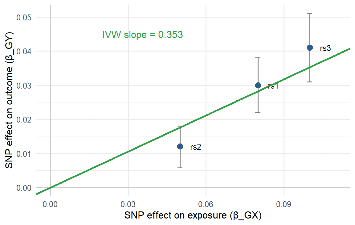
Plot each SNP as a point: x = SNP effect on the exposure, y = SNP effect on the outcome.
The slope of a line through the origin is the causal effect.
IVW is a weighted mean of the per-SNP Wald ratios. The weights are typically

\[w_j = \frac{\beta_{X_j}^2}{SE(\beta_{Y_j})^2}\]

A SNP gets a large weight if it moves the exposure a lot (strong instrument) and its outcome effect is precisely estimated. The same number comes out of a weighted regression of \(\beta_Y\) on \(\beta_X\) through the origin with weights \(1/SE(\beta_Y)^2\) (derivation in 6.7).

IVW on the slide table

SNP	Wald ratio β_Y/β_X	Weight β_X²/SE_Y²	Weight × ratio
rs1	0.030/0.08 = 0.375	0.0064/0.000064 = 100.0	37.50
rs2	0.012/0.05 = 0.240	0.0025/0.000036 = 69.4	16.67
rs3	0.041/0.10 = 0.410	0.0100/0.000100 = 100.0	41.00
Sum		269.4	95.17

\(\hat\beta_{IVW} = 95.17 / 269.4 = 0.353\), with (fixed-effect) \(SE = 1/\sqrt{269.4} = 0.061\). rs2, the weakest instrument, pulls the least.

The slides’ three SNPs as an MR scatter plot (±1 SE of the outcome). The IVW estimate is the slope of the weighted line through the origin.

9.7 Interpreting an MR estimate: units, and “genetically predicted ≠ intervention”

The unit of the exposure decides what the number means. The slides use systolic blood pressure (SBP) as the exposure and pulse wave velocity (PWV, m/s) as the outcome:

Exposure unit	Estimate	Reading
per 1 mmHg SBP	1.05	per 1 mmHg higher SBP, PWV is 5% higher
per 1 SD SBP (e.g. 120 → 126 mmHg)	1.2	per 1 SD higher SBP, PWV is 20% higher

Both describe the same biology on different exposure scales. Always state the unit.

Check the arithmetic: 1 mmHg vs 10 mmHg

The slide continues “per 10 mmHg, PWV increase 50%”. That is the additive approximation (10 × 5%). If 1.05 is a ratio per mmHg, effects multiply: \(1.05^{10} = 1.63\), i.e. +63% per 10 mmHg. The two agree only for small changes. The same logic applies to odds ratios: an OR of 1.2 per SD becomes \(1.2^2 = 1.44\) for 2 SD, not 1.4.

Genetically predicted exposure ≠ intervention effect

Highlighted in red on the slides. Genotype acts from conception, so an MR estimate reflects a lifelong difference in the exposure, and lifetime exposure builds risk. A drug started at age 60 changes the exposure for a much shorter time. MR estimates are therefore often larger than what an intervention in adulthood achieves, and the direction is the more reliable part.

9.8 Pleiotropy, sensitivity analyses and practical pitfalls

Horizontal pleiotropy does not disappear in two-sample MR. Add sensitivity estimates next to the main IVW result:

Method	What it adds
IVW	Main estimate; assumes all instruments valid (or pleiotropy balanced)
Weighted median	Tolerates some invalid instruments (valid if ≥ ~50% of the weight is valid)
MR-Egger	Free intercept; intercept ≠ 0 = directional pleiotropy
Leave-one-out	Rerun leaving out one SNP at a time: is one SNP driving the result?
Heterogeneity	Do the SNP-specific Wald ratios differ more than chance allows?

(Details on weighted median and MR-Egger: 6.8.)

Practical problems specific to two-sample MR (slides):

Problem	What it is	Direction of bias
Weak instruments + non-overlapping samples	SNPs explain little of the exposure	Toward the null
Sample overlap	Some individuals are in both GWAS	Toward the confounded observational estimate
Winner’s curse	SNP effects are overestimated in the discovery data set that selected them	β_GX too large → Wald ratio too small → toward the null
Different populations	True associations may not transport between populations	Unpredictable

More on winner’s curse (GWAS primer): it is common for highly polygenic traits, where many variants with small effects sit just above the significance threshold; effects “close to the discovery threshold tend to be overestimated”. The gold standard correction is to re-estimate the effects in an independent replication cohort with no shared or related individuals. In MR this is why instruments are ideally selected in one sample and their β_GX taken from another.

Why weak instruments behave differently with and without overlap. A weak SNP’s β_GX is mostly noise. In two independent samples the noise in β_GX is unrelated to β_GY, so the ratio is diluted toward zero. When the same people are in both GWAS, the same confounding that links X and Y in those people leaks into both betas, pulling the estimate toward the ordinary (confounded) observational association.

Toward zero, as with any weak instrument

Toward the confounded observational estimate

Away from zero in the opposite direction

Not biased, since overlap only affects SEs

With complete overlap, weak-instrument bias pulls toward the confounded observational association. With no overlap it pulls toward the null.

Makes β_GX too small and inflates the MR estimate

Changes the sign of β_GX for about half of the SNPs

Makes β_GX too large and shrinks the MR estimate

Only affects the outcome GWAS, not the exposure

SNPs that pass the threshold tend to be the ones whose β happened to come out high. A too-large denominator gives a too-small Wald ratio, biasing toward the null.

Part 2: Polygenic risk scores

9.9 PRS vs MR: same GWAS, different question

	Mendelian randomization	Polygenic risk score
Question	Does variation in X causally affect Y?	Can genetic information predict who is at higher risk?
Level	Population: one causal estimate	Individual: one score per person
Uses	A few strong, valid instruments	Many SNPs, including weak ones
Pleiotropy	A threat (exclusion restriction)	Fine: any predictive signal helps

Association → causal inference → prediction. A GWAS finds variants associated with a trait. MR uses them to test causation. A PRS asks: even if each effect is small and each variant is common, what if we add many variants together? “PRS takes us back to the individual again.”

Definition (course book, quoting the tutorial): a PRS is a “single value estimate of an individual’s genetic liability to a phenotype, calculated as a sum of their genome-wide genotypes, weighted by corresponding genotype effect size estimates derived from GWAS data”. The terms genetic risk score (GRS), polygenic score (PGS) and PRS are used interchangeably. The book gives a GRS two goals: to predict the likelihood of developing a disease, and to estimate how much predictive capacity the associated variants capture.

Why many variants? Most complex traits are polygenic (the LDL exercise found > 100 SNPs acting through many genes), and most SNPs have a tiny effect by themselves. Most people carry some risk alleles. Only the sum separates people meaningfully.

9.10 The PRS formula

A PRS is calculated for an individual \(i\) as the sum over \(M\) SNPs of allele dosage × estimated effect:

\[PRS_i = \sum_{j=1}^{M} G_{ij}\,\hat\beta_j\]

where \(G_{ij} \in \{0, 1, 2\}\) is the number of effect alleles person \(i\) carries at SNP \(j\), and \(\hat\beta_j\) comes from the GWAS.

Slide example. \(\hat\beta_1 = 0.10\), \(\hat\beta_2 = -0.15\), \(\hat\beta_3 = 0.05\), \(\hat\beta_4 = 0.15\).

ID	SNP1	SNP2	SNP3	SNP4	PRS
1	0	2	0	1	0.10·0 − 0.15·2 + 0.05·0 + 0.15·1 = −0.15
2	0	1	2	0	0.10·0 − 0.15·1 + 0.05·2 + 0.15·0 = −0.05
3	1	0	0	0	0.10
4	0	1	0	1	−0.15 + 0.15 = 0.00

(IDs 3 and 4 are not computed on the slide.) Person 3 has the highest score. A negative β (SNP2) means the allele lowers risk, so carrying it lowers the score.

For a binary disease the β’s are log-odds ratios, so the PRS is on the log-odds scale and relative risks multiply across SNPs (tutorial).

9.11 Two datasets: discovery and target

A PRS analysis (preferably) needs two data sets:

	Discovery sample (tutorial: base data)	Target / validation sample
Provides	The β estimates (GWAS summary statistics)	Individual genotypes, the phenotype/outcome, covariates
Typical size	Very large (a consortium GWAS)	Smaller cohort where the score is computed and tested

The course book describes the same split as base data (GWAS summary statistics) and target data (“an independent sample from the base data used for PRS analysis”), and stresses that the effect allele and genotyping method must be known and equal in both (course book).

The two must be independent (tutorial; also course book and GWAS primer: “accuracy measurements can be inflated if the discovery GWAS and the target cohort share individuals”). If people from the target sample were also in the discovery GWAS, their own outcomes helped estimate the β’s, and the PRS–outcome association in the target sample is inflated. This is the PRS version of the sample-overlap problem in 9.8. Close relatives across the two samples cause a milder version of the same inflation.

Other checks from the tutorial’s QC list: confirm which allele is the effect allele in the base GWAS (otherwise the score points the wrong way), remove ambiguous (palindromic) and duplicated SNPs, use the same genome build, and prefer target samples of ≥ 100 individuals.

9.12 Choosing SNPs: clumping + thresholding, and shrinkage

Two problems with using raw GWAS output directly:

Many estimates are imprecise. Most SNP β’s are mostly noise, and the top hits are inflated by winner’s curse.
Linkage disequilibrium. Strongly correlated SNPs carry the same signal. Summing them counts one locus many times, which is “not good in prediction models”.

The classical approach: clumping + thresholding (C+T).

Clumping: keep the lead SNP from each locus (as in Step 1 of MR).
Thresholding: include SNPs with a GWAS p-value below a threshold, and typically try several thresholds (e.g. \(5\times10^{-8}\), \(10^{-5}\), \(10^{-3}\), 0.01, 0.05, 0.1, 0.5, 1) and keep the one that predicts best (tutorial).

Common confusion: weak instruments are a problem in MR but welcome in a PRS. Now we may include weak instruments, “remember the weak learners from stat learning!” Each SNP adds a little signal; no single SNP needs to be valid on its own, only the sum needs to predict. Pleiotropy does not matter either.

The statistical learning route (slides):

Instead of forcing independence by clumping, estimate the correlation between SNPs and put it into the model (LD-aware methods).
Use LASSO (penalized regression) with a train/test split: SNPs with large effects that are partly sampling noise are shrunk toward zero. This directly counteracts winner’s curse.

The GWAS primer calls C+T “pruning and thresholding”, “the simplest and most practical method”; more complex methods model the LD structure or add functional information to estimate the effects better (GWAS primer). The course book lists penalized regression (LASSO or ridge) and Bayesian approaches, which also handle LD, and warns that they must be tuned to avoid overfitting (course book).

C+T includes a SNP at its full β or excludes it (β set to 0). Shrinkage methods keep more SNPs but pull every β toward zero by an amount depending on how noisy it is (tutorial).

Overfitting the threshold

If you try 10 thresholds in the target data and report the best one, that “best” R² or AUC is optimistic. Choose the threshold in one part of the data and report performance in another (a validation set or cross-validation) (tutorial).

9.13 Interpreting and evaluating a PRS

What a PRS means (slides):

A PRS has no natural unit. It is a relative measure, usually close to normally distributed and often standardized (mean 0, SD 1), so results read “per SD of PRS” or “top 5% vs the rest”.
It does not directly translate into a probability of disease. A high score says “higher risk than others”, not “a 30% risk”.
Most often a PRS predicts less than age, sex, SBP etc.

How to evaluate it (slides):

Question	Measure
Does it add to discrimination?	AUC: the probability that a random case has a higher predicted risk than a random control (0.5 = coin toss, 1 = perfect)
Is it calibrated?	Do predicted risks match observed risks (e.g. predicted 10% → about 10% get the disease)?
Does it add to prediction?	Compare `age + sex + smoking + SBP` with `age + sex + smoking + SBP + PRS`: the gain in AUC (or R², the incremental R² in the tutorial) is what the PRS adds

The model comparison written out (GWAS primer):

\[H_0:\ \text{Phenotype} \sim \text{covariates} + e \qquad H_1:\ \text{Phenotype} \sim \text{PRS} + \text{covariates} + e\]

with covariates such as age, sex and ancestry (principal components). The variance explained by the PRS term alone is the difference between the two models: \(R^2\) for a continuous trait, a pseudo-\(R^2\) from logistic regression for a binary one.

What the course material adds about accuracy:

Point	Source
AUC > 0.75 is considered informative for screening; > 0.99 is needed as a diagnostic aid. Calibration curves check for overfitting	course book
The maximum possible accuracy is capped by the SNP-based heritability of the trait	GWAS primer
One of the best PRSs (glaucoma): top decile has 4.2-fold higher risk than the bottom 90%	GWAS primer
A high odds ratio per SD does not mean good screening: at a 5% false-positive rate, a published CAD PRS would miss 85% of people who develop the disease. Reclassification measures (e.g. the net reclassification index) are more clinically relevant than OR or AUC	GWAS primer
Accuracy decays with ancestral distance from the discovery GWAS (mostly European), because allele frequencies and LD differ	GWAS primer, course book
Clinical utility is “yet to be established”; ethical, legal and social issues, e.g. genetic determinism and stigma	course book, GWAS primer

Why the added value is usually small. The PRS is partly correlated with the traditional risk factors (e.g. a PRS for CAD partly works through LDL and SBP), so part of its signal is already in the base model.

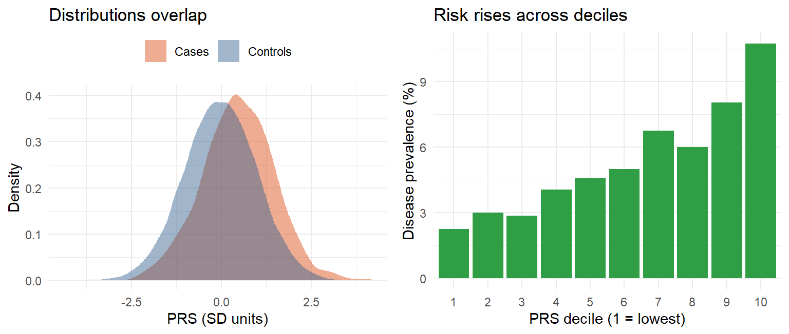
Simulated data (not from the slides). Left: the PRS distributions of cases and controls overlap heavily, so the score cannot sort individuals well on its own. Right: yet disease prevalence rises steeply across PRS deciles, so the score does separate groups.

Reading the figure (tutorial, Fig. 5): in real data (BMI PRS in UK Biobank, explaining ~5% of BMI variance) the prevalence of severe obesity rises steeply in the top strata, but most obese individuals still have an average or low PRS. A high-risk group can be identified; an individual cannot be predicted with confidence.

The PRS is not associated with CAD at all

It adds little discrimination beyond the base model

The base model is badly calibrated and useless

The PRS is a better predictor than age and sex

An association can be clearly significant while the gain in AUC is small. Part of the PRS signal is already carried by the traditional risk factors.

A has a 2% absolute risk of developing the disease

A will develop the disease, since +2 SD is extreme

A’s genetic liability is high relative to others

A’s risk is exactly twice the population average

A PRS is relative. +2 SD places A in roughly the top 2.5% of scores; turning that into an absolute risk needs a calibrated model with the baseline risk.

Part 3: Extra material, a real study that uses both

9.14 Extra material: remnant cholesterol, LDL and CHD in UK Biobank

Extra material, not required reading

This study was provided as extra material, separate from the course’s reading material. It is included because it applies the lecture’s methods to real data. The section has no exam flag.

(extra material) Björnson E, Adiels M, Taskinen M-R, Burgess S, Rawshani A, Borén J, Packard CJ (2023). “Triglyceride-rich lipoprotein remnants, low-density lipoproteins, and risk of coronary heart disease: a UK Biobank study.” European Heart Journal 44:4186–4195. A Gothenburg study that uses almost every tool from Lectures 4–9 and continues the course’s LDL story.

The question. Triglyceride-rich lipoproteins (TRL) and their partly digested remnants also carry cholesterol and one apoB per particle, like LDL. Is a remnant particle more atherogenic per particle than an LDL particle, or is CHD risk simply a function of the number of apoB particles?

Design, mapped to the course:

Step in the paper	Course concept
GWAS in UK Biobank (~350,000 people not on lipid-lowering therapy), adjusted for age, sex and genetic PCs 1–5	GWAS covariates, population stratification (4.4)
SNPs with P < 5×10⁻⁸, MAF > 0.01, LD-pruned at r² < 0.1 (20 Mb window)	Instrument selection, clumping (9.3)
SNPs associated with lipoprotein(a) removed (28 SNPs) → 1125 SNPs	Guarding against a known horizontal pleiotropic pathway
Multivariable MR with IVW: several exposures (apoB, LDL-C, TRL/remnant-C) in one model, each effect adjusted for the others	Extension of IVW (9.6)
Exposure allele defined as the apoB-raising allele	Orienting SNPs before estimation (9.5)
SNPs split into two clusters by their ratio of effect on TRL/remnant-C vs apoB	Using the scatter of SNP effects, as in the MR plot
Polygenic scores per cluster, SNP weights from ridge regression, cohort split into PGS deciles; Cox model gives HR per SD apoB	PRS construction and shrinkage (9.10, 9.12)
Sensitivity: LD thresholds r² < 0.01 and < 0.001; robust IVW, MR-Egger, MR-Lasso	Sensitivity analyses (9.8)
Replication: UK Biobank exposure β’s combined with CHD β’s from CARDIoGRAMplusC4D (1049 of 1125 SNPs)	This replication is a two-sample MR (9.1)

Key results:

Result	Number
Multivariable MR, OR for CHD per 1 mmol/L: TRL/remnant-C vs LDL-C	2.59 (1.99–3.36) vs 1.37 (1.27–1.48)
The same per population SD (TRL/remnant-C SD 0.30 mmol/L, LDL-C SD 0.82 mmol/L)	1.36 vs 1.29
OR per SD apoB, cluster 1 (receptor pathway: PCSK9, LDLR, APOB; low remnant/LDL ratio 0.19)	1.33 (1.26–1.40)
OR per SD apoB, cluster 2 (lipolysis: LPL, APOC3, ANGPTL4; high remnant/LDL ratio 0.59)	1.76 (1.58–1.96)
Replication in CARDIoGRAMplusC4D, cluster 1 vs cluster 2	1.44 vs 1.68
Cluster PGS in a Cox model, HR per SD apoB, cluster 1 vs cluster 2	1.45 vs 1.94

Conclusion of the paper: per apoB particle, the risk is about twice as large when the genetic effect runs through remnants rather than LDL, so TRL/remnants appear substantially more atherogenic per particle than LDL.

The unit lesson from 9.7, in real numbers

Per mmol/L, remnant cholesterol looks far more harmful than LDL-C (OR 2.59 vs 1.37; on the log-odds scale 0.95 vs 0.31, three times as large). Per SD, the two are close (1.36 vs 1.29). Both are correct: 1 mmol/L is more than 3 SD of remnant-C but only about 1.2 SD of LDL-C. Check: \(2.59^{0.30} \approx 1.33\) and \(1.37^{0.82} \approx 1.29\), matching the per-SD odds ratios up to rounding. Always ask “per what?” before comparing MR estimates.

Reading it critically (with Lecture 9 in mind):

Mostly one-sample. Exposure β’s and CHD outcomes both come from UK Biobank, so the samples overlap. With weak instruments that biases toward the observational estimate (9.8), and the SNPs were selected and weighted in the same data (winner’s curse). The two-sample replication in CARDIoGRAMplusC4D, an independent outcome data set, addresses exactly this, and gave similar cluster ORs.
IVW assumes all 1125 SNPs are valid. The authors report that robust IVW, MR-Egger and MR-Lasso agreed closely, and removed Lp(a)-associated SNPs up front.
Ancestry: mainly white European, so results may not transport (9.4, 9.13).
Measurement: remnant-C was not measured directly but computed as non-HDL-C − LDL-C, and remnant apoB was not measured at all; per-particle atherogenicity was inferred from the SNP clusters.
MR ≠ intervention (9.7): the ORs describe lifelong genetic differences, not what a drug lowering remnants in adulthood would achieve.

It raised the number of SNPs from 1049 to 1125

Its outcome data are independent of the exposure GWAS

It measured remnant apoB directly, unlike UK Biobank

It removed the need for the three MR assumptions

Combining UK Biobank exposure β’s with CHD β’s from an independent consortium is a two-sample MR. It avoids sample overlap, which in the one-sample analysis could bias estimates toward the confounded association. The assumptions still apply.

Remnant-C is twice as harmful per SD as LDL-C

Per SD the two effects are of similar size

LDL-C is more harmful per mmol/L than remnant-C

The ORs cannot be compared on any common scale

Per SD: 2.59^0.30 ≈ 1.33 and 1.37^0.82 ≈ 1.29 (the paper reports 1.36 and 1.29). The large difference per mmol/L reflects the different spreads of the two measures.

Practice

Two-sample MR and PRS in R

Runs in your browser. The MR numbers are the slides’ table; the PRS evaluation uses simulated data.

Tasks

Which SNP needed harmonising in Part A? What would the IVW estimate be if you forgot to flip it?
Which SNP has the lowest F? Is it a weak instrument?
In Part B, which person has the highest PRS, and why does carrying SNP2 lower the score?
In Part C, how much does the PRS add to the AUC? Change the PRS coefficient in risk_log_odds from 0.4 to 1.0 and rerun. What happens?

Model answer

rs4: the exposure effect allele is C, the outcome file reports T. Its outcome β becomes +0.020 per C (Wald ratio 0.33, in line with the others). Without flipping, rs4’s Wald ratio is −0.33 and it pulls the IVW estimate down, from about 0.35 to about 0.13.
rs2 and rs3 both have F = 25, rs4 has F = 36, rs1 has F = 64. All are above 10, so none is weak by the rule of thumb.
id3 (0.10). SNP2’s β is −0.15, so each copy subtracts 0.15: its effect allele lowers risk.
The AUC rises only by a few hundredths with a coefficient of 0.4 (OR ≈ 1.5 per SD), even though the PRS is strongly significant. With 1.0 (OR ≈ 2.7 per SD) the gain is clearly larger. Added discrimination depends on how much of the risk the score explains, not on its p-value.

Why-questions

Why is two-sample MR so widely used if it needs extra care?

It needs only published summary statistics, so it can use the largest GWAS available for both the exposure and the outcome, without access to individual data. The extra care (matching, harmonisation, comparable populations) is bookkeeping, and the three MR assumptions are the same as in one-sample MR.

Why must alleles be harmonised before computing the Wald ratio?

β means “per copy of the effect allele”, and the two GWAS may have chosen different effect alleles. Dividing betas that refer to different alleles gives a ratio with the wrong sign, which can reverse the causal conclusion.

Why is winner’s curse a bias toward the null in MR?

Instruments are selected because their exposure β passed a threshold, and those that pass tend to have β’s that happened to come out high. An overestimated β_GX is the denominator of the Wald ratio, so the causal estimate becomes too small.

Why can a PRS include weak and pleiotropic SNPs when MR cannot?

MR needs every instrument to satisfy the causal assumptions, because one invalid SNP biases the causal estimate. A PRS only has to predict: each SNP adds a little signal, like the weak learners in an ensemble, and it does not matter by which pathway the SNP acts.

Why must the discovery and target samples be independent?

If target individuals were in the discovery GWAS, their own outcomes shaped the β’s used to score them. The score then partly “remembers” their outcomes, and the association in the target sample is inflated, the same way training error is optimistic in statistical learning.

Why does an MR estimate not equal the effect of a drug?

The genetic variant shifts the exposure from conception, so MR estimates the effect of a lifelong difference. A treatment started in adulthood acts for a shorter time, so its effect is usually smaller even when MR is right about causality.

Spaced review

Relevance

Independence

Exclusion restriction

None; only vertical pleiotropy does

Horizontal pleiotropy gives the SNP a path to the outcome that bypasses the exposure, violating the exclusion restriction.

Approximately independent lead SNPs, one per signal

All SNPs that pass genome-wide significance

Only the SNPs that are rare in the reference panel

The SNPs with the largest effect sizes per chromosome

Clumping keeps the most significant SNP and removes those correlated with it, so the remaining SNPs carry separate signals.

The change per copy of the other (non-effect) allele

The change per copy of the effect allele

The difference between homozygotes of either allele

The correlation between the SNP and the trait

Under the additive model β is the change in the trait (or log-odds) per copy of the effect allele. That is why harmonisation needs to know which allele it is.