Martin’s key concepts
The 20 concepts on the key-concepts list for GWAS, Mendelian randomization and proteomics, one module each
On 2 October the course published Martin’s key concepts, a list of 20 concepts for the GWAS, Mendelian randomization (MR) and proteomics part of the course (Lectures 4–6, 8 and 9). When the lecture pages were written this list did not exist, so the material is spread across many sections and some concepts only got a sentence or two.
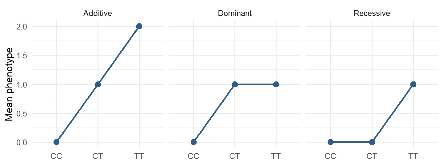
This page collects the list into 20 short modules, in the list’s own order. Each module gives an exam-ready definition you can say in one or two sentences, the common confusion to avoid, a quick check, and links to the lecture sections that go deeper. Three concepts that were thin in the lectures get more space here: additive, dominant and recessive models (K.4), colocalization (K.19) and biomarker vs causal protein (K.20).
Mark each module Reviewed or Confident as you go. The status is saved in this browser and counted on the dashboard under 🔑.
NoteSource and what changed in the rest of the app
Source: “Martins part key_concepts.docx” (course material, uploaded 2 October), a list of 20 concept names without further text. The definitions, examples and questions on this page are written for this app.
Changes elsewhere: lecture sections that cover these concepts now carry the badge 🔑 Martin’s key concepts instead of ❔ or 🗣️. Seminar topics (🗣️) are no longer described as “not on the written exam”: seminar content can also come on the exam. The seminar’s own questions are on Seminar questions.
Part 1: From SNP to GWAS
K.1 SNP (single-nucleotide polymorphism)
- Usually biallelic: two alleles, often called the reference/other and the effect allele in GWAS files.
- “Polymorphism” traditionally means common enough to be a normal variant in the population (often minor allele frequency ≥ 1%). A rare change in one family is usually called a variant or mutation.
- SNPs are what SNP arrays genotype and what GWAS tests, one at a time.
Don’t confuse: a SNP is a position with variation in the population; an allele is one of the possible bases at that position; a genotype is the pair of alleles one person carries.
Deeper: 3.3c dbSNP and rs numbers · 4.2 SNPs, alleles, MAF
A deletion of one gene that only some people carry
A single base position where alleles differ between people
A mutation that arises in a tumour but not in the germline
The one allele that a person has at a given position
A SNP is a position with variation across the population. One person’s pair of alleles at it is their genotype.
K.2 Genotype and allele dosage (0/1/2)
| Genotype (effect allele = T) | CC | CT | TT |
|---|---|---|---|
| Dosage | 0 | 1 | 2 |
- Imputed SNPs give an expected dosage between 0 and 2 (for example 1.7), because the genotype is predicted with uncertainty.
- The dosage only means something once you know which allele is counted. Swap the effect allele and every dosage becomes 2 − dosage, and β changes sign.
Don’t confuse: dosage counts the effect allele, which is not always the minor allele or the “risk” allele.
Deeper: 4.4 The additive model · A3 Reading association output
2, because the person has two copies of an allele
1, because G is the other allele at this SNP
0, because the person has no copies of A
It cannot be coded without knowing the MAF
Dosage counts copies of the effect allele. GG has zero A alleles, so dosage = 0.
K.3 Minor allele frequency (MAF)
- Computed from genotype counts: each heterozygote contributes one copy, each homozygote two. With \(n_{AA}, n_{Aa}, n_{aa}\): \(f_a = (2n_{aa} + n_{Aa}) / (2N)\).
- Low MAF means low power: few people carry the allele, so β is estimated with a large SE. Rare variants are why GWAS QC often filters on MAF.
- MAF is population-specific. The minor allele in Europeans can be the major allele in another ancestry, which matters when combining datasets (seminar question on GLGC vs 1000 Genomes).
Don’t confuse: MAF is not the same as the effect allele frequency (EAF). If the effect allele is the major allele, EAF = 1 − MAF.
Deeper: 4.2 SNPs, alleles, MAF and genotype frequencies · 3.9 Hardy–Weinberg
0.04, the share of people who are TT
0.36, the share of people who carry a T
0.20, the share of all alleles that are T
0.80, the share of all alleles that are C
T alleles = 2 × 40 + 320 = 400 out of 2,000 alleles = 0.20. T is the less common allele, so MAF = 0.20.
K.4 Additive, dominant and recessive models
Coding of the same SNP under the three models (effect allele = T)
| Model | CC | CT | TT | What β means |
|---|---|---|---|---|
| Additive | 0 | 1 | 2 | Change in phenotype per extra copy of T |
| Dominant (T dominant) | 0 | 1 | 1 | Difference between carriers (one or two T) and non-carriers |
| Recessive (T recessive) | 0 | 0 | 1 | Difference between TT and everyone else |
Why GWAS use the additive model (Lecture 4, “Worth noting 2”): you test a million SNPs and do not know each one’s true pattern. The additive model is the simple default; it has reasonable power even when the true pattern is dominant or recessive, and it uses one degree of freedom. Dominant and recessive models are useful when you study one specific SNP or gene in depth.
Don’t confuse: dominance describes the genotype–phenotype relationship, not the allele. The same allele can act dominant for one phenotype and recessive for another (Lecture 4).
Deeper: 4.4 The additive model · 3.6 Mendelian genetics
Each extra copy of T is compared with one fewer copy
People with at least one T against people with no T
People with two copies of T against everyone else
Heterozygotes against both kinds of homozygote
Recessive coding is 0/0/1: only TT is coded 1, so β is the difference between TT and the CC + CT group.
Dominant, since one copy has the full effect
Additive, since each copy adds one unit
Recessive, since only TT differs from CC
None, since the heterozygote should lie halfway
CT already has the same mean as TT, so one copy is enough: a dominant pattern (0/1/1). An additive pattern would give about 4.0, 4.5, 5.0 or 4, 5, 6.
K.5 Genome-wide association study (GWAS)
- Hypothesis-free: no candidate gene is chosen in advance.
- Output: one β, SE and p per SNP (summary statistics, K.11), shown as a Manhattan plot (position vs −log₁₀ p) and checked with a QQ plot.
- Continuous phenotype → linear regression (β = mean difference per allele); binary → logistic regression (β = log-odds per allele, OR = e^β).
- A GWAS finds associations. The top SNP is usually a tag in LD with the causal variant, and the association can still be confounded (population structure).
Don’t confuse: GWAS finds loci, not genes or mechanisms. Going from a hit to biology needs fine-mapping, QTL data, colocalization, MR or experiments.
Deeper: 4.6 The GWAS scan · 4.9 Population structure · 4.10 From hit to biology · 5.2 The full GWAS pipeline
To increase the number of SNPs that can be tested
To adjust for ancestry differences that can confound
To convert the additive model into a dominant one
To remove SNPs that are in strong LD with each other
If allele frequencies and the phenotype both differ between ancestry groups, SNPs look associated because of ancestry. The PCs capture ancestry and remove that confounding.
K.6 Effect size, standard error and p-value
Example. β = 0.05 SD per allele, SE = 0.008.
| Step | Value |
|---|---|
| z = β / SE | 0.05 / 0.008 = 6.25 |
| Two-sided p | ≈ 4 × 10⁻¹⁰, below 5 × 10⁻⁸ |
| 95% CI | 0.05 ± 1.96 × 0.008 = 0.034 to 0.066 |
- SE shrinks with larger sample size, higher MAF and lower phenotype variance. That is why a tiny β can have a tiny p in a large GWAS.
- Binary outcome: β is a log(OR). OR per allele = e^β; for two copies under the additive model, OR = e^(2β).
- p measures evidence, not importance. A highly significant SNP can explain almost none of the phenotype variance.
Don’t confuse: a small p-value does not mean a large effect. Compare β (and its units) to judge size.
Deeper: 4.3 Phenotype types and the per-allele effect · 4.4 β, SE and p
SNP 2 has a larger effect on the phenotype
SNP 2 has a higher MAF or a larger sample
SNP 2 lies closer to the gene it regulates
SNP 2 was tested with the dominant model
SE depends on sample size, allele frequency and phenotype variance. With β the same, a smaller SE comes from more information: more people or more carriers of the allele.
K.7 Genome-wide significance
\[\frac{0.05}{1\,000\,000} = 5 \times 10^{-8}\]
- “Independent” is the key word: there are many more SNPs than that, but because of LD neighbouring SNPs are correlated, so the effective number of independent tests in European-ancestry genomes is about one million.
- It controls the family-wise error rate: the chance of even one false positive across the whole scan is about 5%.
- SNPs with 5 × 10⁻⁸ < p < 10⁻⁵ are sometimes called “suggestive”.
Don’t confuse: passing the threshold does not make a SNP causal, and failing it does not mean “no effect”; it may mean too little power.
Deeper: 4.7 Multiple testing, Manhattan and QQ plots · 7.11 FWER vs FDR · 7.12 Bonferroni
It is the p-value of the strongest SNP in the first GWAS
0.05 divided by about a million independent tests
0.05 divided by the total number of SNPs on an array
It is the FDR level that Benjamini–Hochberg gives
Bonferroni: α / m with m ≈ 10⁶ independent tests, after accounting for LD. It is a FWER threshold, not an FDR threshold.
K.8 Linkage disequilibrium (LD; r²)
- LD exists because nearby SNPs are inherited together: recombination between them is rare, so the haplotypes they sat on are preserved over generations.
- r² = 1: one SNP perfectly predicts the other, so they give the same GWAS signal. r² ≈ 0: independent.
- LD is population-specific. Compute it in a reference panel that matches the ancestry of the GWAS (for example the European part of 1000 Genomes).
- LD generally decays with distance, but physical distance is not LD: two close SNPs can have low r², and LD blocks vary in size.
Don’t confuse: linkage is about co-inheritance within families (recombination frequency); LD is the correlation of alleles across a population.
Deeper: 3.7 Linkage, recombination and LD · 4.8 Lead SNP and r² · 5.4b r² bands
A similar association, since B almost copies A
No association, because only one SNP can be causal
An association in the opposite direction from A
An association only if B lies inside a gene’s exon
With r² = 0.95, B’s alleles nearly predict A’s, so B shows almost the same signal. That is why GWAS hits appear as towers of correlated SNPs.
K.9 Lead SNP and GWAS locus
- A locus is defined around the lead SNP, by a distance window (for example ± 500 kb) and/or by LD with the lead SNP.
- The lead SNP is the best statistical tag, not necessarily the causal variant. The causal variant can be any SNP in strong LD with it, or one that was not genotyped at all.
- One locus can contain more than one independent signal (conditional analysis or clumping can reveal a secondary signal).
Don’t confuse: “lead SNP” (strongest p in the region) ≠ “causal SNP” (the variant that changes the biology) ≠ “nearest gene” (often assumed, not proven).
Deeper: 4.8 Lead SNP and r² · 4.10 Locus, lead SNP, QTLs · 5.4 Finding the causal SNP
Because the lead SNP is always in a non-coding region
Because SNPs in strong LD with it give nearly the same p
Because the lead SNP is chosen by its position in the gene
Because causal variants never reach genome-wide significance
Many SNPs in high LD carry almost the same signal, and the smallest p among them can be partly chance or better genotyping. The causal variant may be another SNP in LD or an unmeasured one.
K.10 LD clumping and independent genetic signals
The algorithm
| Step | Action |
|---|---|
| 1 | Sort significant SNPs by p, smallest first |
| 2 | Take the top SNP as an index SNP |
| 3 | Remove SNPs within the window (for example 1,000 kb) with r² above the threshold (for example 0.01–0.1) |
| 4 | Repeat with the next remaining SNP until none are left |
- Why: correlated SNPs carry the same information. For MR you need independent instruments, otherwise the same signal is counted several times and the SE is too small. For PRS clumping avoids double-counting.
- Choices matter: a wider window compares more SNP pairs (slower, catches long-range LD, leaves fewer SNPs); a lower r² threshold removes more SNPs (stricter independence).
- More SNPs can survive clumping than there are causal variants: two weakly correlated tags of one causal variant can both pass a lenient threshold, and SNPs outside the window are never compared.
Don’t confuse: “independent” (low r² between the kept SNPs) is not “causal”. Each clump still represents a region.
Deeper: 5.4b r² bands and LD clumping · A5 Manual LD clumping · Seminar S.1 and S.5
Clumping makes every instrument genome-wide significant
Correlated SNPs would count one signal several times
Clumping removes the need to harmonise the alleles
IVW can only handle one SNP per chromosome at most
IVW treats each SNP as independent evidence. SNPs in LD repeat the same signal, so the estimate gets falsely precise.
K.11 GWAS summary statistics
- Before using them, check four things: which allele is the effect allele, whether β is OR or log(OR), the scale of the phenotype (SD units? log?), and the genome build (hg19/GRCh37 vs hg38/GRCh38).
- LD cannot be computed from summary statistics: they have no genotypes per person. Use a reference panel with matching ancestry.
- Two-sample MR needs two sets: one for the exposure, one for the outcome, matched on SNP and allele.
Don’t confuse: summary statistics are per SNP, not per person. You cannot rerun the regression with new covariates from them.
Deeper: 4.6 Summary statistics · 5.5 LD with summary statistics · 9.2 The data you need
Reading off the β and p of a given SNP
Finding SNPs below p = 5 × 10⁻⁸
Estimating r² between two SNPs for clumping
Converting a log-odds β into an odds ratio
r² needs the genotypes of individuals. Summary statistics have none, so LD comes from a reference panel such as 1000 Genomes.
Part 2: Mendelian randomization
K.12 Instrumental variable (IV)
flowchart TD
  Z["Z (instrument)"] --> X["X (exposure)"]
  X --> Y["Y (outcome)"]
  U["U (confounders)"] --> X
  U --> Y
- The idea comes from econometrics. The classic example is the randomization in an RCT: the coin flip shifts treatment and is independent of everything else.
- In MR the instrument is a genetic variant: alleles are allocated at conception, before the exposure and the disease, and independently of most lifestyle confounders.
Don’t confuse: an IV is not a confounder or a covariate to adjust for. Its job is to give variation in the exposure that confounders do not touch.
Deeper: 6.3 Genetic variants as instruments · 6.4 Why we need MR: confounding
The outcome measured at the end of follow-up
The confounders recorded at the baseline visit
The random allocation to treatment or control
The treatment the participant actually took
Allocation shifts the treatment received and is independent of confounders, just like an allele in MR. The treatment actually taken is the exposure.
K.13 Mendelian randomization (MR)
- “Nature’s randomized trial”: people who inherited exposure-raising alleles are, on average, like people who were randomized to a slightly higher exposure for life.
- One-sample MR: exposure and outcome in the same people. Two-sample MR: SNP–exposure and SNP–outcome effects from two different GWAS, using only summary statistics.
- The answer is the effect per unit of genetically predicted exposure, which is lifelong and usually small; it is not the same as the effect of a drug given in middle age.
Don’t confuse: MR is only as good as its three assumptions (K.14). A significant MR estimate with a pleiotropic instrument is not causal evidence.
Deeper: 6.4 Why we need MR · 9.1 Two-sample MR · 9.7 Interpreting an MR estimate
Because the outcome GWAS is always run before the exposure GWAS
Because MR uses only SNPs located inside the exposure’s gene
Because the disease cannot change the inherited genotype
Because the Wald ratio is always positive for causal effects
The genotype is fixed at conception. Disease can change measured biomarkers but not the alleles, so the arrow cannot run from outcome to instrument.
K.14 The three MR assumptions
| # | Assumption | How you check it | Typical threat |
|---|---|---|---|
| 1 | Relevance | p < 5 × 10⁻⁸ in the exposure GWAS; F-statistic > 10 | Weak instruments |
| 2 | Independence | Cannot be proven; adjust for ancestry, check associations with known confounders | Population stratification, assortative mating, selection |
| 3 | Exclusion restriction | Cannot be proven; biology of the gene, MR-Egger intercept, weighted median, outlier tests | Horizontal pleiotropy |
- Only assumption 1 can be tested directly. Assumptions 2 and 3 are made plausible, never proven, which is why MR uses several sensitivity analyses.
Don’t confuse: “the SNP is associated with the outcome” is not an assumption. That is what MR tests, and it is only interesting if the three assumptions hold.
Deeper: 6.5 The three MR assumptions · 6.8 Sensitivity analyses · 9.3 F-statistic
Relevance, from the SNP–exposure association
Independence, from the SNP–outcome association
Exclusion restriction, from the MR-Egger slope
None of them, since all three are untestable
Relevance is visible in the exposure GWAS (p-value, F-statistic). Independence and exclusion restriction involve unmeasured paths and can only be made plausible.
K.15 Horizontal vs vertical pleiotropy
Causal diagrams (each arrow means “directly affects”):
flowchart TD
  S1["SNP"] --> L1["LDL-C"]
  L1 --> A1["atherosclerosis"]
  A1 --> C1["CHD"]
flowchart TD
  S2["SNP"] --> L2["LDL-C"]
  L2 --> C2["CHD"]
  S2 --> I2["inflammation"]
  I2 --> C2
  linkStyle 2,3 stroke:#c92a2a,stroke-width:2px,stroke-dasharray:6 4,color:#c92a2a
- Horizontal pleiotropy shows up as instruments whose Wald ratios disagree with the rest, an MR-Egger intercept away from zero, or IVW and weighted median giving different answers.
- trans-pQTLs and SNPs in genes with many functions are the usual suspects. cis instruments in the exposure’s own gene reduce the risk.
Don’t confuse: vertical pleiotropy is not a problem to remove. It is the causal chain MR is designed to detect.
Deeper: 6.6 Pleiotropy · 6.8 MR-Egger and weighted median · 9.8 Pleiotropy and pitfalls
Vertical pleiotropy, which does not bias the estimate
Horizontal pleiotropy, which can bias the estimate
A weak-instrument problem under the relevance assumption
Reverse causation from stroke to blood pressure
The SNP reaches stroke through BMI, a path that does not go through blood pressure. That is horizontal pleiotropy and breaks the exclusion restriction.
K.16 Wald ratio and inverse-variance weighted (IVW) MR
\[\hat\beta_{\text{Wald}} = \frac{\beta_{\text{SNP}\to Y}}{\beta_{\text{SNP}\to X}}, \qquad SE_{\text{Wald}} \approx \frac{SE_{\text{SNP}\to Y}}{|\beta_{\text{SNP}\to X}|}\]
\[\hat\beta_{\text{IVW}} = \frac{\sum_j \beta_{X_j}\beta_{Y_j}/SE_{Y_j}^2}{\sum_j \beta_{X_j}^2/SE_{Y_j}^2}\]
Example. Three clumped SNPs (exposure in mmol/L, outcome log-odds).
| SNP | β exposure | β outcome | SE outcome | Wald ratio |
|---|---|---|---|---|
| 1 | 0.20 | 0.10 | 0.02 | 0.50 |
| 2 | 0.10 | 0.06 | 0.02 | 0.60 |
| 3 | 0.30 | 0.12 | 0.03 | 0.40 |
IVW numerator = (0.20·0.10 + 0.10·0.06)/0.0004 + 0.30·0.12/0.0009 = 65 + 40 = 105. Denominator = (0.04 + 0.01)/0.0004 + 0.09/0.0009 = 125 + 100 = 225. IVW = 105/225 ≈ 0.47 log-odds per mmol/L, OR ≈ e^0.47 ≈ 1.6.
- Before computing: harmonise the alleles so both β refer to the same effect allele, and for a binary outcome use log(OR).
- Through the origin = assumes no horizontal pleiotropy (zero exposure effect → zero outcome effect). MR-Egger frees the intercept to test that.
Don’t confuse: the Wald ratio is per unit of the exposure’s scale. An exposure in SD units and one in mmol/L give different numbers for the same biology.
Deeper: 6.7 The Wald ratio and IVW · 9.5 Harmonisation · 9.6 Wald ratio and IVW
Because the exposure GWAS centres all β values at zero
Because a SNP with no exposure effect should have no outcome effect
Because weighting by precision removes the intercept term
Because it makes the estimate robust to pleiotropic SNPs
Under the exclusion restriction the only way a SNP affects the outcome is through the exposure, so zero on X must give zero on Y. A non-zero intercept (MR-Egger) suggests directional pleiotropy.
Part 3: Proteomics and genetics
K.17 Proteomics and protein abundance
- Why proteins: they do the work in cells, change with disease, diet, drugs and age, and are the targets of most drugs.
- Why it is hard: plasma protein concentrations span about 10 orders of magnitude, so a few abundant proteins (albumin, immunoglobulins) dominate; one gene can give several proteoforms (isoforms, post-translational modifications).
- Platforms: affinity-based (Olink, SomaScan: antibodies or aptamers, thousands of proteins, relative units) and mass spectrometry (peptides, can see isoforms and give absolute amounts with internal standards).
- NPX is relative and log₂: +1 NPX = twice as much of that protein in that sample. It cannot be compared between different proteins.
Don’t confuse: abundance ≠ function. A variant can change what a protein does without changing how much there is, and an affinity assay can miss a form it does not bind.
Deeper: 8.1 Why study the proteome · 8.4 Three technology families · 8.5 Units and NPX · 8.13 Reading: comparing eight platforms
Sample B has about four times as much protein X
Sample B has 2 units/mL more protein X than sample A
Sample B has more protein X than any protein in sample A
Sample B’s protein X is more biologically active
NPX is log₂, so a difference of 2 = 2² = 4-fold for the same protein. It says nothing about other proteins or about activity.
K.18 pQTLs: cis-pQTL and trans-pQTL
| cis-pQTL | trans-pQTL | |
|---|---|---|
| Location | Near the protein’s own gene | Far away (> 500 kb) or another chromosome |
| Likely mechanism | Direct: transcription, splicing, stability, secretion of that protein | Indirect: transcription factors, receptors, pathways |
| As MR instrument | Preferred: clear biology, less pleiotropy | Higher risk of horizontal pleiotropy |
- Found with a GWAS that has the protein level as the phenotype: protein = β₀ + β₁ × dosage + ε.
- Caution: a coding (missense) cis variant can change the epitope an antibody or aptamer binds and fake a pQTL: lower measured signal, unchanged amount.
Don’t confuse: cis is defined relative to the protein’s gene, not relative to any gene. A SNP next to gene A that changes protein B is trans for B.
Deeper: 8.9 pQTLs · 8.10 Protein MR · 8.11 Challenges of protein MR
A cis-pQTL, a good candidate MR instrument
A trans-pQTL, with a high risk of pleiotropy
A cis-pQTL, which proves ABC causes disease
An eQTL, since it is near a gene’s promoter
Near the protein’s own gene → cis. cis-pQTLs are preferred instruments for protein MR, but the three MR assumptions and colocalization still need checking.
K.19 Colocalization
The logic from the slides (Lecture 8): compare the pattern of association across the region for the protein and for the disease. If one shared variant drives both, SNPs in LD with it produce the same shape of signal for both traits: the same SNPs are strongest, and the association weakens in step as LD with the shared variant falls.
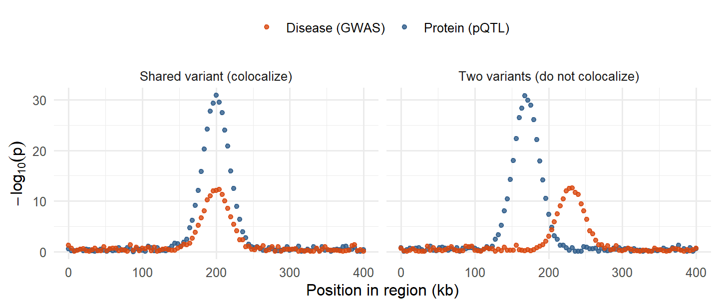
Why MR alone is not enough: if SNP A raises the protein and a different SNP B in LD with A raises disease risk through another mechanism, an MR using A will still find a “protein → disease” effect. That is LD confounding. Colocalization checks for it.
NoteBeyond the slides: the formal coloc method
The widely used Bayesian method (the R package coloc) compares five hypotheses for a region: H0 no association with either trait, H1 only trait 1, H2 only trait 2, H3 both traits but different causal variants, H4 both traits and one shared causal variant. It reports a posterior probability for each, and PP.H4 above about 0.8 is often taken as evidence of colocalization. It needs only summary statistics for both traits in the region. The slides describe the idea; this formal version is background, not course material.
Don’t confuse: “both signals are in the same locus” is not colocalization. Two causal variants 50 kb apart can sit in one locus with overlapping towers of association.
Deeper: 8.11 Challenges of protein MR (colocalization) · 8.12 From association to mechanism
The protein causes the disease, since the signals overlap
Two different causal variants drive the two signals
The pQTL must be a trans-pQTL for the protein P
The disease GWAS must be confounded by ancestry
If one variant drove both, the same SNPs would be strongest for both traits. Mismatched peaks point to distinct causal variants, so an MR through P here may reflect LD, not causation.
K.20 Biomarker vs causal protein
| Biomarker | Causal protein | |
|---|---|---|
| Question | Does it predict or reflect disease? | Does changing it change disease? |
| Evidence | Association, prediction (AUC), reproducibility | MR with cis-pQTLs, colocalization, experiments, trials |
| Useful for | Diagnosis, prognosis, risk prediction, monitoring treatment | Drug targets, understanding mechanism |
| Example type | Troponin after heart damage: excellent marker, consequence not cause | A protein whose cis-pQTL predicts disease in MR and colocalizes |
- A protein associated with disease in a PWAS can be (1) a cause, (2) a consequence of disease (reverse causation), or (3) a correlate sharing a confounder (smoking, BMI, inflammation).
- A good biomarker does not have to be causal; a causal protein is not always a good biomarker (it may vary little between people or be hard to measure).
- The route from biomarker to causal protein (Lecture 8): association → pQTL → MR and colocalization → experiments (CRISPR, cell models, animal models).
Don’t confuse: “strongly associated” and “predictive” do not mean “causal”. Lowering a consequence-marker does not undo the disease.
Deeper: 1.3b Biomarkers and their five roles · 8.7 PWAS · 8.8 Association is still not causation · 8.12 From association to mechanism
It causes heart attacks and should be a drug target
It is a useful biomarker, but may not be causal
It must have a strong cis-pQTL in the general population
It proves that MR would find a causal effect on CHD
Rising after the event suggests it is a consequence (like troponin). Prediction makes it a useful biomarker; causality needs MR, colocalization or experiments.