flowchart TD
  G["GWAS SNP (tag)"] -.-|"LD: inherited together"| C["causal variant"]
  C -->|"affects"| P["phenotype"]
Lecture 3 — Recap, Mutations and Genetics
miRNA vs siRNA · PCSK9 drugs · HGVS nomenclature · germline vs somatic · sequencing · Mendel · LD · SNP arrays · Hardy–Weinberg
This lecture moves from how one gene works to how variation in genes is described, measured and inherited. It starts with small RNAs that switch genes down (miRNA and siRNA) and the two drug types that hit PCSK9 from different sides. Then it teaches the formal notation used to write a mutation down precisely, the difference between inherited and acquired mutations, and the technologies used to read DNA.
The second half is classical genetics with a statistical eye: Mendel’s laws, what happens when two genes sit close together on a chromosome (linkage), and the population-level version of that, linkage disequilibrium (LD). LD is the single concept that makes GWAS results tricky to interpret in Lectures 4–6, so it is worth understanding here.
The lecture ends with Hardy–Weinberg equilibrium (HWE): simple probability that tells you what genotype frequencies to expect from an allele frequency. You will use the same \(p^2\), \(2pq\), \(q^2\) logic again in Lecture 4.
NoteSources and session
Slides: “Lecture 3_recap and mutations.pdf” (8 Sep 2026) and “Lecture 3_genetics.pdf” (9 Sep 2026). The two files overlap in the second half; the content is merged here.
Session boundary warning. The course’s reading guide says “Lecture 3_genetics.pdf” was actually presented at the start of the Lecture 4 session, as a recap (“the same lecture notes as posted for lecture 3”). So Sections 3.6–3.9 here (Mendel, LD, SNP arrays, HWE) were taught in the Lecture 4 session, right before “Lecture 4 from SNP to GWAS.pdf”. This matters if an exam question refers to material “from lecture 4”.
Rough plan: Week 2, day 1. Genetic variation and protein function.
3.1 Recap and non-coding RNA genes
Quick recap of Lecture 2 (restated because the instructor treats it as foundational):
| DNA | RNA | |
|---|---|---|
| Strands | Double-stranded, antiparallel | Usually single-stranded |
| Direction of synthesis | 5′ → 3′ | 5′ → 3′, antiparallel to its DNA template |
| Primer needed? | Yes (DNA polymerase) | No (RNA polymerase) |
Beyond mRNA, rRNA and tRNA, two more classes of non-coding RNA genes exist. These genes are transcribed into RNA but never translated; the RNA itself is the functional product.
- snRNA (small nuclear RNA): involved in RNA splicing, removing non-coding sections from a pre-mRNA before translation.
- miRNA (microRNA): regulates gene expression (next section).
3.2 miRNA and siRNA
| miRNA (microRNA) | siRNA (small interfering RNA) | |
|---|---|---|
| Length | About 22 nucleotides | About 21–23 nucleotides |
| Origin | Encoded in the genome | Derived from double-stranded RNA |
| Binding to target mRNA | Imperfect match | High complementarity (near-perfect) |
| Mechanism | Inhibits translation or promotes mRNA degradation | Cleavage and degradation of the target mRNA |
| Number of targets | Many genes at once | One specific gene |
| Use | Natural regulation; broadly dysregulated in cancer (Lecture 7) | Designed drugs and experimental gene silencing |
The “one miRNA, many targets” property is why miRNA dysregulation shows up across cancers and is the centerpiece of Lecture 7’s case study. The precise matching of siRNA is why it works as a designed therapeutic: it silences exactly the gene you choose.
siRNA is encoded in the genome, so the body already makes it
siRNA pairs almost perfectly with one target mRNA only
siRNA blocks translation of hundreds of mRNAs at once
siRNA is longer than miRNA, so it binds more strongly
siRNA binds its target with high complementarity and triggers cleavage of that one mRNA. miRNA binds imperfectly and therefore regulates many mRNAs at once, which is useless for targeting a single gene.
3.2b Two drugs, one pathway: Leqvio vs Repatha/Praluent
Leqvio (inclisiran): an siRNA drug that lowers LDL cholesterol.
- It targets PCSK9 mRNA in liver cells and causes it to be degraded.
- Less PCSK9 protein is made.
- PCSK9 normally promotes LDLR degradation, so more LDL receptors stay on liver cells.
- More LDLR means more LDL-C cleared from the blood.
Delivery: the siRNA is chemically linked to a sugar called GalNAc, which binds ASGPR receptors, highly expressed on liver cells (hepatocytes). The GalNAc–siRNA complex is taken up into the liver cell, the siRNA is released and loaded into a protein complex that finds and degrades PCSK9 mRNA. GalNAc works as an “address label” that sends the drug to the liver rather than the whole body.
Repatha (evolocumab) and Praluent (alirocumab): monoclonal antibodies, proteins engineered to bind one specific target. They bind free circulating PCSK9 protein in the blood and stop it from binding LDL receptors on liver cells. More LDLR stays available.
| Leqvio (inclisiran) | Repatha / Praluent | |
|---|---|---|
| Drug type | siRNA | Monoclonal antibody |
| Target | PCSK9 mRNA in hepatocytes | PCSK9 protein in blood |
| Effect on PCSK9 | Stops it being made | Blocks its action |
| Delivery | GalNAc → ASGPR on liver cells | Circulates and binds free PCSK9 |
| End result | More LDLR → lower LDL-C | More LDLR → lower LDL-C |
Take-away: there can be more than one druggable point along a single pathway.
It is the active part that binds and degrades PCSK9 mRNA
It is an antibody that blocks circulating PCSK9 protein
It binds ASGPR, steering the siRNA into liver cells
It raises LDL receptor synthesis directly in hepatocytes
GalNAc is a sugar that binds ASGPR receptors on hepatocytes, so the siRNA is taken up by the liver. It acts as an address label; the siRNA does the silencing.
3.3 Gain and loss of function: the PCSK9 variants
A mutation can make a protein work better (gain of function, GoF) or worse (loss of function, LoF).
NoteLearn the concept, not the example
Gain of function and loss of function are on the professor’s list. The PCSK9 variants below are only the course’s running example: the lecturer said not to learn specific mutations or medicines.
| Variant | DNA | Protein | Classification | Effect |
|---|---|---|---|---|
| D374Y | c.1120G>T |
p.Asp374Tyr |
Point mutation, SNV, missense, GoF | PCSK9 binds LDLR much more strongly → more LDLR degraded → higher LDL-C, higher CVD risk |
| F216L | c.646T>C |
p.Phe216Leu |
GoF | |
| S127R | c.381T>A |
p.Ser127Arg |
GoF | |
| Y142* | c.426C>G |
p.Tyr142* (= p.Tyr142Ter) |
Point mutation, SNV, nonsense, LoF | Premature stop (“Ter” = terminator) |
| R97del | c.290_292delGCC |
p.Arg97del |
In-frame deletion, LoF | 3 nt removed, frame kept, arginine 97 missing |
What phenotype would a PCSK9 LoF mutation give? Work it through the pathway: less functional PCSK9 → less LDLR degradation → more LDLR → more LDL cleared → lower LDL-C and lower cardiovascular risk. This is exactly what the PCSK9 drugs mimic pharmacologically. D374Y (GoF) goes the opposite way.
Indels are “a bit more tricky to annotate”: note the _ range and the del keyword instead of the > used for substitutions.
Higher, because PCSK9 no longer clears LDL from the blood
Lower, because fewer LDL receptors are degraded
Unchanged, because PCSK9 does not affect LDL receptors
Higher, because LDL receptors are degraded more quickly
PCSK9 promotes LDLR degradation. Losing PCSK9 function leaves more LDLR, more LDL is cleared, and LDL-C falls. PCSK9 inhibitor drugs imitate this LoF effect.
3.3b HGVS nomenclature and reference sequences
Which reference is a variant described against? The PCSK9 annotations above use the transcript NM_174936.4 from NCBI RefSeq.
| Part | Meaning |
|---|---|
NM |
Curated mRNA transcript |
174936 |
Accession number identifying this gene’s transcript |
.4 |
Version 4 of the reference sequence; references are revised, so using the wrong version can shift coordinates |
NM_174936.4:c.1120G>T, also written NM_174936.4(PCSK9):c.1120G>T, reads: in the PCSK9 transcript NM_174936.4, at coding DNA position 1120, G is replaced by T.
HGVS nomenclature (Human Genome Variation Society) is the international standard for describing variants in DNA, RNA and protein. A complete description always states which sequence (reference identifier) and what change at what position.
| Reference prefix | Sequence type | Position prefix | Coordinate system | |
|---|---|---|---|---|
NM_ |
mRNA | c. |
Coding DNA (numbered from start of coding sequence) | |
NC_ |
Genomic (e.g. a whole chromosome) | g. |
Genomic DNA (numbered from start of chromosome/contig) | |
NP_ |
Protein | p. |
Protein (amino acid position) |
D374Y written at all three levels
| Level | Notation |
|---|---|
| DNA (coding) | NM_174936.4:c.1120G>T or NM_174936.4(PCSK9):c.1120G>T |
| Protein | NP_777596.2:p.Asp374Tyr or NP_777596.2(PCSK9):p.Asp374Tyr |
| Genomic, GRCh38 | NC_000001.11:g.55057454G>T |
| Genomic, GRCh37 | NC_000001.10:g.55523127G>T |
The same biological variant has different genomic coordinates under GRCh37 and GRCh38. That is why the genome build always matters.
Protein position 1120 changed from glycine to threonine
Coding DNA position 1120 in transcript version 4, G to T
Chromosome 1 position 1120 in genome build 4, G to T
mRNA number 1120 of gene 174936, deleted from G to T
NM_ = mRNA reference, .4 = version, c. = coding DNA coordinates, 1120G>T = position 1120, G replaced by T. A protein change would use p. and amino acid codes (p.Asp374Tyr).
3.3c dbSNP, rs numbers and genome builds
dbSNP is an NCBI database (separate from RefSeq) cataloguing SNPs and other short variants, including indels. Every variant gets a stable identifier, an rs number (Reference SNP ID).
- D374Y,
NM_174936.4(PCSK9):c.1120G>T, is rs137852912. - dbSNP maps it to chromosome 1, position 55057454 (GRCh38), equivalently 55523127 (GRCh37/hg19).
GRCh37 = Genome Reference Consortium Human build 37. hg19 is the UCSC Genome Browser’s name for essentially the same assembly. The names are used almost interchangeably, so do not be confused when you see both.
Two more real examples (genes relevant to blood cancers)
| Gene | Coding / protein | GRCh37 genomic | Reference → mutated |
|---|---|---|---|
| RUNX1 | NM_001754.5(RUNX1):c.594T>G, p.(Asp198Glu) |
g.36231790A>C |
CTCGGGGCCC[A]TCCACTGTGA → CTCGGGGCCC[C]TCCACTGTGA |
| PHF6 | NM_032458.3(PHF6):c.635G>T, p.(Cys212Phe) |
g.133547902G>T |
AGGCCTAAAT[G]TGGATTTTGC → AGGCCTAAAT[T]TGGATTTTGC |
Note for RUNX1: the coding change is T>G but the genomic change is A>C. The gene lies on the minus strand of the chromosome, so the genomic (plus-strand) letters are the complements of the coding letters.
3.4 Germline vs somatic mutations
A clean side-by-side comparison on the slides, a typical definition-style exam question.
| Germline mutations | Somatic mutations | |
|---|---|---|
| Origin | In egg or sperm cells (germ cells) | Acquired during life, in non-reproductive cells |
| Distribution | In the DNA of every cell in the body | Confined to the affected tissue/tumor |
| Inheritance | Can be passed to offspring | Cannot be passed to offspring |
| Detection | Routine blood or saliva test | Needs a biopsy/sample of the diseased tissue |
| Clinical impact | Inherited disorders, hereditary cancer syndromes | Cancers and localized benign tumors |
Worked example: AML (acute myeloid leukemia), explicitly not a solid tumor, follows the somatic pattern:
| AML | |
|---|---|
| Origin | Acquired during life, in bone marrow stem cells |
| Distribution | Leukemic blood cells and bone marrow |
| Inheritance | Cannot be inherited |
| Detection | Bone marrow aspirate or peripheral blood sample |
| Clinical impact | Uncontrolled production of abnormal white blood cells |
How AML diagnostics uses NGS (next-generation sequencing), a template for finding a somatic mutation in a patient:
- Identify somatic mutations specific to the leukemic cells (present in cancer cells, absent in the patient’s normal cells).
- Design PCR primers to amplify a small region around the candidate mutation.
- Sequence that region across many cells.
- Do we find the mutation, and at what VAF (variant allele frequency), the fraction of reads/cells carrying the mutant allele?
VAF measures prevalence within one patient’s cells (useful for tumor burden and clonal evolution). It is not the population allele frequency of Section 3.6/Lecture 4. The approach is targeted deep sequencing: amplify → prepare → sequence one small region, giving very high read depth there, which is needed to detect a mutation present in only some cells.
Somatic, acquired in the tumor tissue during life
Germline, inherited from one of the parents
Germline, because it was found in a biopsy
Somatic, and so it can be passed to children
A germline mutation would be in every cell, including blood. Found only in the tumor → somatic. Somatic mutations are not passed on to offspring.
3.5 Sequencing and genotyping technologies
Sequencing determines the actual order of nucleotides in a piece of DNA.
| Method | Characteristics |
|---|---|
| Sanger sequencing | The original method: individual reactions, highly accurate, lower throughput, longer reads |
| NGS (next-generation sequencing) | Many reactions in parallel: fast and cheap per base, but shorter reads (about 50–300 nucleotides) |
Genotyping (as distinct from sequencing) determines which allele(s) a person carries at already known variant positions, without sequencing the surrounding DNA from scratch. TaqMan SNP genotyping is a PCR-based technology for doing this efficiently at a single known SNP. SNP arrays (Section 3.8) genotype up to millions of known SNPs at once.
3.6 Mendelian genetics: vocabulary and laws
Genetics is the study of how genes and traits pass from parents to offspring. Gregor Mendel found the basic principles by breeding pea plants and studying single-gene traits (seed shape, flower color, plant height).
Core vocabulary (exactly what short-answer questions target):
| Term | Definition |
|---|---|
| Locus (pl. loci) | A specific physical position on a chromosome |
| Homologous chromosomes | The two copies of essentially the same chromosome, one from each parent |
| Allele | An alternative version (DNA sequence) found at a particular locus |
| Genotype | An individual’s genetic makeup: which alleles they carry |
| Phenotype | The observable trait that results (in part) from the genotype |
| Dominant allele (B) | Affects the phenotype when at least one copy is present |
| Recessive allele (b) | Affects the phenotype only with two copies |
| Homozygous | Two identical alleles: BB (homozygous dominant), bb (homozygous recessive) |
| Heterozygous | Two different alleles: Bb |
Mendel’s three laws
- Law of Dominance: in a heterozygote the dominant allele determines the phenotype and the recessive allele is masked (Bb → dominant phenotype).
- Law of Segregation: an organism carries two alleles per gene, but they separate during gamete formation so each gamete gets only one (Bb → B gametes or b gametes, never both).
- Law of Independent Assortment: alleles of different genes are inherited independently of each other, except when the genes lie close together on the same chromosome (linkage, next section).
The person shows the recessive phenotype because b is present
Each gamete from this person carries either B or b, not both
The person’s gametes all carry both B and b in equal amounts
Alleles of B and of other genes are always inherited together
Segregation: the two alleles separate into different gametes, so each gamete carries one. The phenotype (dominant) is the Law of Dominance; inheritance across genes is Independent Assortment.
3.7 Linkage, recombination and linkage disequilibrium
Recombination (crossover) happens during meiosis: homologous chromosomes exchange segments. This is what lets alleles of genes on the same chromosome be reshuffled.
Genetic linkage. Genes physically close on the same chromosome are linked: they tend to be inherited together, because a crossover is less likely to land in the short stretch between them. The closer, the stronger the linkage; the farther apart, the more likely recombination separates them. Test crosses measure recombination frequency and estimate genetic distance.
\[r = \frac{\text{number of recombinant offspring}}{\text{total offspring}}, \qquad 0\% \le r \le 50\%\]
- \(r = 0\%\): complete linkage, always inherited together.
- \(r = 50\%\): behaves as unlinked (different chromosomes or far apart). 50% is the ceiling because that is what independent assortment alone produces.
Linkage disequilibrium (LD) is central from Lecture 4 to Lecture 6, so understand it here. LD is the non-random association of alleles at different loci in a population: some combinations of alleles occur together more (or less) often than chance predicts. Loci close together tend to show high LD because recombination has had fewer chances to separate them. Recombination erodes LD over generations, but LD stays strong over the short distances relevant for most GWAS.
Detecting LD: compare the observed frequency of a haplotype (a specific combination of alleles at two or more loci on the same chromosome copy) with the frequency expected if the loci were independent. Observed ≈ expected → little or no LD. Observed ≠ expected → LD.
Worked example. Two biallelic loci: Locus 1 has A/a, Locus 2 has B/b. Frequencies: \(P(A) = 0.5\), \(P(B) = 0.4\).
| Step | Calculation |
|---|---|
| Expected AB frequency if independent | \(P(A) \times P(B) = 0.5 \times 0.4 = \mathbf{0.20}\) |
| Observed AB haplotype frequency | From real data, say 0.30 |
| Conclusion | 0.30 ≠ 0.20 → the loci are in LD. The difference \(D = 0.30 - 0.20 = 0.10\) is the classic LD coefficient. |
The measure \(D\) and the correlation-based \(r^2\) (Lecture 4–5) are standard ways to quantify LD; the slides use observed vs expected directly and \(r^2\) later.
Strong LD, because 0.18 is much lower than 0.9
No LD, because 0.18 equals 0.3 × 0.6
Complete linkage, because both alleles are common
LD cannot be judged without the recombination rate
Expected under independence: 0.3 × 0.6 = 0.18. Observed equals expected, so there is no evidence of LD.
3.8 First look at GWAS, and SNP arrays
GWAS (genome-wide association study) searches the entire genome for variants associated with a trait or disease. Millions of SNPs are compared between individuals with different phenotypes; for each SNP you ask: is one allele more common among people with the trait?
Where LD comes in. A SNP that is significant in a GWAS is not necessarily the causal variant. Nearby variants are often in LD, so a significant SNP may simply be correlated with (“tag”) the real causal variant:
A GWAS can show a strong association for “SNP A” even though “SNP B” does the biological work, just because A and B are inherited together.
SNP arrays (SNP chips) genotype hundreds of thousands to millions of known SNP positions at once. At a SNP such as rs12345 with alleles A or G, the array determines whether a person is AA, AG or GG.
Mechanism: the array holds many short DNA probes, each recognizing DNA with one particular allele. The person’s DNA is fragmented and allowed to hybridize (bind) to the probes; fluorescent signals show which probes bound.
flowchart TD
  A["DNA sample"] --> B["fragment the DNA"]
  B --> C["let fragments bind (hybridize)<br/>to probes on the SNP array"]
  C --> D["detect which probes light up"]
  D --> E["genotype (e.g. AA, AG or GG)"]
If both the “A signal” and the “G signal” light up at a position, the person is an AG heterozygote.
3.9 Hardy–Weinberg equilibrium
HWE gives the expected genotype frequencies in a population when allele frequencies stay constant across generations. The idealized assumptions: no selection, no new mutation, no migration, random mating, infinite population size. (The slides focus on the math rather than the full assumption list.)
For a locus with two alleles, A (frequency \(p\)) and a (frequency \(q\)):
\[p + q = 1\]
With random mating, each gamete carries A with probability \(p\) or a with probability \(q\), independently:
\[P(AA) = p^2, \qquad P(Aa) = 2pq, \qquad P(aa) = q^2, \qquad p^2 + 2pq + q^2 = 1\]
The heterozygote term is \(2pq\) because there are two ways to get Aa: A from mother and a from father, or the reverse.
| \(p\) = P(A) | \(q\) = P(a) | \(p^2\) (AA) | \(2pq\) (Aa) | \(q^2\) (aa) |
|---|---|---|---|---|
| 0.9 | 0.1 | 0.81 | 0.18 | 0.01 |
| 0.7 | 0.3 | 0.49 | 0.42 | 0.09 |
| 0.5 | 0.5 | 0.25 | 0.50 | 0.25 |
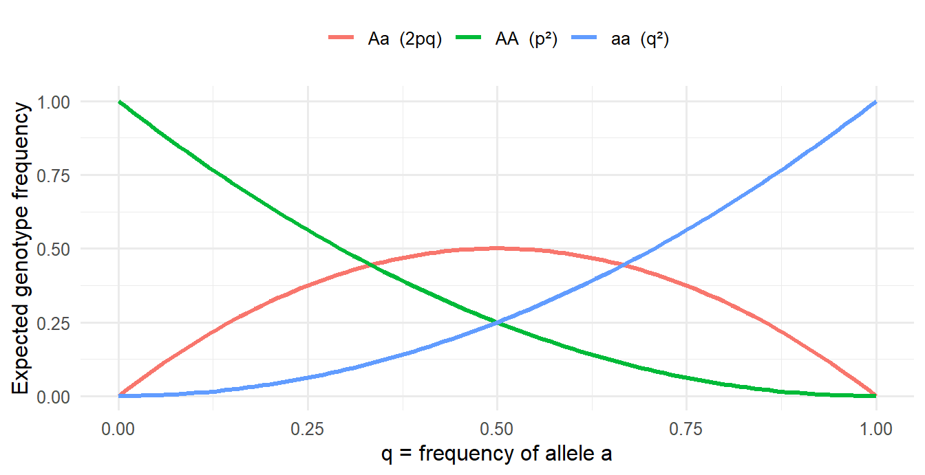
The same binomial logic is used in Lecture 4 (MAF → genotype frequencies). In practice, observed genotype counts that deviate strongly from HWE are a quality-control check on genotyping data.
0.04
0.16
0.32
0.64
p = 0.8, q = 0.2. 2pq = 2 × 0.8 × 0.2 = 0.32. (0.04 is q², 0.64 is p², 0.16 is pq without the factor 2.)
Practice
NoteHardy–Weinberg and an HWE check in R
Runs in your browser. The first run takes a few seconds while R loads.
Tasks
- What are \(p\) and \(q\) here? Are the observed counts consistent with HWE?
- Change the counts to
AA = 500, Aa = 200, aa = 300. What happens to the HWE test, and what would you suspect in real genotyping data? - Use the LD example: with \(P(A) = 0.5\) and \(P(B) = 0.4\), compute the expected AB haplotype frequency and \(D\) if the observed frequency is 0.30.
TipModel answer
- \(p = (720 + 480)/2000 = 0.6\), \(q = 0.4\). Expected: 360, 480, 160, exactly the observed counts, so \(\chi^2 = 0\) and the SNP is in HWE.
- \(p = 0.6\) again but far too few heterozygotes (expected 480, observed 200). \(\chi^2\) is huge and the p-value tiny. In genotyping data this suggests a technical problem (e.g. heterozygotes being miscalled) or population structure, so the SNP would be flagged in QC.
0.5 * 0.4= 0.20 expected;D <- 0.30 - 0.5 * 0.4= 0.10, evidence of LD.
Why-questions
TipWhy does recombination frequency top out at 50%, not 100%?
Unlinked loci are assorted independently: a gamete has a 50% chance of carrying a “recombinant” combination just by chance. Recombination between linked loci can only push them toward that independent state, never past it.
TipWhy is the top GWAS SNP not automatically the causal one?
Because of LD. All SNPs correlated with the causal variant show an association too. The strongest one might just be the best-measured tag, or the causal variant might not even be on the array.
TipWhy does the same variant have two different genomic positions?
Positions are counted against a reference genome build. GRCh37 (hg19) and GRCh38 are different assemblies, so chromosome 1 is numbered differently in each: rs137852912 is at 55523127 in GRCh37 and 55057454 in GRCh38. The rs number stays the same.
TipWhy is VAF different from allele frequency?
VAF is the fraction of reads (cells) within one patient’s sample that carry a mutation, used to track a tumor clone. Allele frequency (or MAF) is how common an allele is across people in a population.
Spaced review
Silent
Missense
Nonsense
Frameshift
UAG is a stop codon, so the protein is cut short: a nonsense mutation.
Proteins are fixed at conception, like DNA sequence
Disease itself can change RNA, protein and metabolites
Proteins never influence tissue or organ function
The chain always runs strictly from disease to DNA
The chain is not one-directional: disease can alter RNA, protein and metabolite levels. Only DNA is fixed and cannot be changed by the disease.
Further reading
Links from the course’s reading guide (“Reading links connected to lectures” on Canvas). IB = Introductory Biology (CK-12), GB = General Biology (Boundless), MG = Modern Genetics, all on LibreTexts.
Mutations, PCR and sequencing
- Mutation types: IB chapter 4.8
- Types of mutations and their annotation: Khan Academy
- PCR: Khan Academy
- Sequencing: Khan Academy
Genetics (the genetics part was taught at the start of the Lecture 4 session)
- Genetics, basic concepts: IB chapter 3.4
- Mendel’s Law of Dominance: GB chapter 12.3B (alleles can be dominant or recessive)
- Mendel’s Law of Segregation: GB chapter 12.3C
- Mendel’s Law of Independent Assortment: GB chapter 12.3D
- Recombination and linkage: GB chapter 12.3E, MG chapter 4.2
- Recombination frequency and test crosses: a video linked on Canvas (no address in the reading guide)
- Longer text on linkage and recombination (optional): Introduction to Genetics (Singh), chapter 9
- Hardy–Weinberg equilibrium: MG chapter 11.1
- Examine if a population is in HWE: MG chapter 11.2
NoteCourse files on Canvas (GU login required)