Lecture 4 — From SNP to GWAS

Allele frequency and MAF · additive model · β, SE, OR · covariates · summary statistics · 5×10⁻⁸ · Manhattan and QQ plots · population structure · loci and QTLs

A genome-wide association study (GWAS) is one simple regression repeated about a million times. For each SNP you count how many copies of one allele each person carries (0, 1 or 2), regress the phenotype on that count, and record the effect size, its standard error and a p-value. That is the whole method; everything else in this lecture is about doing it carefully and reading the output correctly.

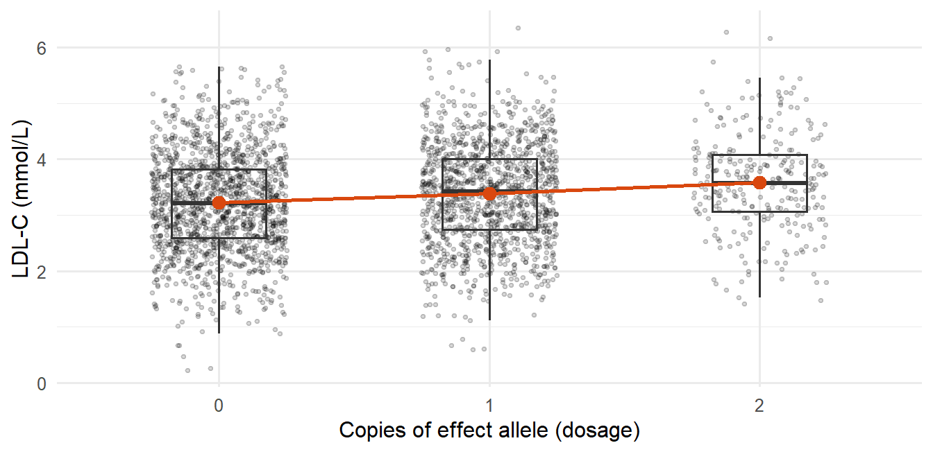
For example, if each copy of an allele raises LDL cholesterol by 0.2 mmol/L on average, the regression slope is 0.2. For a disease outcome you use logistic regression instead, and the slope becomes a log odds ratio.

The intuition to hold on to: genetic effects are usually small compared with everything else that varies between people, but with enough people you can still detect them. Testing a million SNPs at once also means you need a much stricter p-value threshold, and a significant SNP tells you where to look, not what is causal.

This page covers allele and genotype frequencies, the additive model for continuous and binary outcomes, covariates, GWAS summary statistics, multiple testing, Manhattan and QQ plots, why hits come in clusters, population structure and the step from a hit to biology. This lecture is calculation-heavy: be able to redo every worked example with new numbers.

Sources and session

Slides: “Lecture 4 from SNP to GWAS.pdf”. Remember that “Lecture 3_genetics.pdf” (Mendel, LD, SNP arrays, HWE) was presented at the start of this same session as a recap.

Assigned reading: Uffelmann E, Huang QQ, Munung NS, et al. Genome-wide association studies. Nature Reviews Methods Primers 2021;1:59. The most directly relevant academic reading for Lectures 4–6.

Exercise data mentioned (not needed here): Lecture4_ex1.csv and jointGwasMc_LDL.txt, a real LDL-C GWAS summary statistics file (~200 MB), reused in Lecture 5.

Rough plan: Week 2, day 2. From SNP to GWAS.

No instructor EXAM tags in this lecture

None of the Lecture 4 slides carry the “EXAM” marker. The 📌 flags below are inferred: the lecture is built around worked calculations (MAF → genotype frequencies, log β → OR, allele frequency → genotype frequency for rs11591147), so being able to redo them with other numbers is high-priority prep.

4.1 Genotype → phenotype, and why association is not causation

DNA variation can plausibly cause a phenotype (disease status, a biomarker level). The reverse is logically impossible: a phenotype or disease cannot change your inherited DNA sequence, which was fixed at conception, long before any adult disease.

This directional certainty is exactly why genetic variants are useful for causal inference (Mendelian randomization, Lecture 6). But finding a variant associated with a phenotype is still only an association: confounding, chance and linkage can all produce a spurious-looking association, so causality still has to be investigated.

4.2 SNPs, alleles, MAF and genotype frequencies

At a given position, the nucleotide is sometimes A and sometimes C across people: a SNP. You can refer to it by base-pair position or by its rs number. The two possible nucleotides are its alleles.

MAF (minor allele frequency) is the frequency of the less common allele. By convention the minor allele is often called “the mutant”, but that is a labeling choice: the rarer allele is not necessarily the harmful one.

With C as reference, each person carries 0, 1 or 2 copies of the non-reference allele A:

Genotype	Copies of A
CC	0	homozygous reference
CA	1	heterozygous
AA	2	homozygous

Always know which allele is the reference

Flipping the reference allele flips the sign of every downstream effect estimate.

Worked example: MAF → genotype frequencies (the HWE calculation from Lecture 3 applied). MAF = 10%: \(P(A) = 0.1\), \(P(C) = 0.9\).

Genotype	Probability	Frequency	Out of 10,000 people
CC	\(0.9 \times 0.9\)	0.81	≈ 8,100
AC	\(0.9 \times 0.1 + 0.1 \times 0.9\)	0.18	≈ 1,800
AA	\(0.1 \times 0.1\)	0.01	≈ 100

The homozygous-minor group is always the rarest when MAF is low, since its probability is MAF², which shrinks fast.

Worked example: how a genetic effect shows up among cases. Same population. The minor allele doubles the risk of disease Y per copy; baseline risk in CC is 5%.

Genotype	People	Risk	Diseased	Share of all diseased
CC	8,100	5%	≈ 405	67%
AC	1,800	10% (×2)	≈ 180	30%
AA	100	20% (×4)	≈ 20	3.3%
Total	10,000		≈ 605	100%

Frequency of allele A among the diseased: \((180 + 2 \times 20)/(2 \times 605) \approx 18\%\), compared with 10% in the population.

Key takeaway: among people with the disease, the risk allele is enriched relative to the general population. That case–control asymmetry is exactly the signal a GWAS detects.

1,000

800

200

P(minor homozygote) = MAF² = 0.2² = 0.04, and 0.04 × 5,000 = 200. For comparison, heterozygotes are 2 × 0.2 × 0.8 = 0.32, i.e. 1,600 people, and 1,000 is MAF × 5,000, which is not a genotype count.

4.3 Phenotype types and the per-allele effect

Phenotype	Examples	Model
Continuous	Blood pressure, protein concentration, cholesterol, liver fat	Linear regression
Binary	MI yes/no, lung cancer yes/no, disease yes/no	Logistic regression

Per-allele effect. In a large population, group people by how many copies of an allele they carry (0/1/2) and compare the phenotype across groups. Background assumption: other factors that affect the phenotype (lifestyle, etc.) are randomly distributed with respect to genotype. If that fails, you have confounding.

Real example: PNPLA3 rs738409 (I148M) and liver fat. Found in 2009, linked to increased liver fat, roughly 4–5% higher liver fat per copy of the risk allele.

Continuous outcome, linear regression

\[y_i = \beta_0 + \beta_1 \times \text{allele}_i + \varepsilon_i\]

For each extra copy of the effect allele, the phenotype changes by \(\beta_1\) units on average.

Worked example: log-scale β. PNPLA3 rs738409, C→G, “per G allele” \(\beta = 0.08\) in \(\log_{10}\)(liver fat).

Genotype	Log scale	Back-transformed	Interpretation
CG (1 copy)	\(0.08\)	\(10^{0.08} \approx 1.20\)	≈ 20% higher liver fat
GG (2 copies)	\(0.16\)	\(10^{0.16} = 1.2^2 \approx 1.45\)	≈ 45% higher liver fat

On a log scale, effects combine multiplicatively on the original scale: two copies do not double the percentage, they square the factor.

Binary outcome, logistic regression

\[\log\left(\frac{p}{1-p}\right) = \beta_0 + \beta_1 \times \text{allele}\]

Same per-allele interpretation, on the log-odds scale.

Worked example: log-odds β → OR. rs7412, C→T, “per T allele” \(\beta = -0.16\).

Genotype	Log-odds	Odds ratio
CT (1 copy)	\(-0.16\)	\(e^{-0.16} \approx \mathbf{0.85}\)
TT (2 copies)	\(-0.32\)	\(e^{-0.32} \approx \mathbf{0.73}\)

Still not causal

Even with a precise OR, you have not shown causality, mechanism or function, only a statistical association.

1.10

1.22

1.20

0.20

Two copies → 2 × 0.10 = 0.20 on the log-odds scale → OR = e^0.20 ≈ 1.22 (= 1.105²). The per-allele OR is e^0.10 ≈ 1.105.

4.4 The additive model: β, SE and p

The additive model (used for both phenotype types): compare the phenotype across the 0/1/2 groups, with each extra copy one unit of genotype dosage (the X variable).

	Continuous (linear)	Binary (logistic)
β	Mean phenotype difference per extra allele (e.g. +0.2 mmol/L LDL-C, −1.9 mmHg)	Log-odds per allele; OR = exp(β) (β = −0.16 → OR = 0.85)
SE	Precision of β; depends on sample size, allele frequency and phenotype variability	Same dependencies
p-value	Evidence against \(H_0: \beta = 0\)	Evidence against \(H_0: \beta = 0\), i.e. OR = 1.00

“Worth noting” 1: genetic effects are small. The spread of phenotype values within each dosage group (from all the non-genetic factors) is usually much larger than the difference between group means. With a large enough sample you still detect the signal. GWAS is not about finding “the one cause”; hits are clues pointing to proteins involved in physiology or disease.

Simulated LDL-C by genotype dosage with a true effect of +0.2 mmol/L per allele. The group means (red) differ, but the spread within each group is far larger.

“Worth noting” 2: additive, dominant and recessive describe the genotype–phenotype relationship, not the allele. The same allele can act dominant for one phenotype and recessive for another. Most GWAS use additive models because they test many SNPs at once and the additive model is the simplest, most tractable default that works reasonably across all of them. Dominant/recessive models are more useful when studying one specific SNP or gene in depth.

4.5 Covariates

\[y = \beta_0 + \beta_1 G + \beta_2 X_1 + \dots + \beta_n X_{n-1} + \varepsilon\]

\(G\) is genotype dosage; the \(X\)s are covariates such as age, sex, BMI and genetic principal components (PC1, PC2, …).

Why covariates are needed

Population structure. Allele frequency can differ between subpopulations, and the phenotype can also differ between them. Without adjustment you get a spurious SNP–phenotype association driven by structure, not biology (Section 4.9). The genetic principal components capture this.
Age, sex (and BMI). Often strong direct determinants of the phenotype. Adjusting removes their influence and reduces residual noise/confounding.
Technical variables. Genotyping batch, study center, or the batch/method used to measure the phenotype.

β is conditional on the covariates

The same SNP can have a somewhat different β in two studies that adjusted for different covariates. When comparing effect estimates across papers, check what was adjusted for.

4.6 The GWAS scan and summary statistics

GWAS = repeat the single-SNP regression separately for about 1,000,000 SNPs, one model per SNP, each adjusted, giving β, SE and p for every SNP. Conceptually simple but computationally heavy. Software: PLINK and regenie.

Practical notes: HG18 and HG19 are older reference genome versions (compare GRCh37/GRCh38 in Lecture 3). rsIDs refer to fixed variants but are not in genomic-position order, so sorting by rsID does not give positional order.

Standard columns in GWAS summary statistics

Column	Meaning
SNP / rsID	Variant identifier
CHR	Chromosome
BP / POS	Genomic position (base pair)
A1 / EA	Allele 1 / effect allele, the allele β refers to
A2 / OE	The other allele
MAF / EAF	Minor allele frequency / effect allele frequency
Beta / OR	Estimated genetic effect
SE	Standard error
P	p-value
N	Sample size
SNP_hg18	(sometimes) chromosome:position in the hg18 build
Freq.A1.1000G.EUR	(sometimes) frequency of A1 in the 1000 Genomes European reference panel, to cross-check allele frequencies

β in summary statistics is usually the per-A1-allele effect, often in SD units (the phenotype was inverse-normal transformed or standardized first).

Summary statistics contain no individual-level data

Only per-SNP aggregates, which is why they can be shared much more freely than genotype data. When using them, always know: which allele is the effect allele, whether β is OR or log(OR) for binary outcomes, the scale of the phenotype (log? SD units?) and the genome build.

Each C allele lowers LDL-C by 0.05 SD on average

Each T allele lowers LDL-C by 0.05 SD on average

People with the T allele have 5% lower LDL-C in total

The SNP explains 5% of the variance in LDL-C

β is the per-effect-allele (A1) difference. A1 = T, so each extra T is associated with 0.05 SD lower LDL-C. Relative to C the direction is reversed, which is why knowing the effect allele matters.

4.7 Multiple testing, Manhattan and QQ plots

Testing ~1,000,000 SNPs at \(p < 0.05\) would give about \(1{,}000{,}000 \times 0.05 = 50{,}000\) false positives by chance. The field’s standard threshold is:

\[p < 5 \times 10^{-8} \approx \frac{0.05}{1{,}000{,}000}\]

a Bonferroni-style correction for ~1 million independent tests (Bonferroni is formalized in Lecture 7). Significance at this level means a SNP is statistically robust, not that it is biologically important or has a large effect.

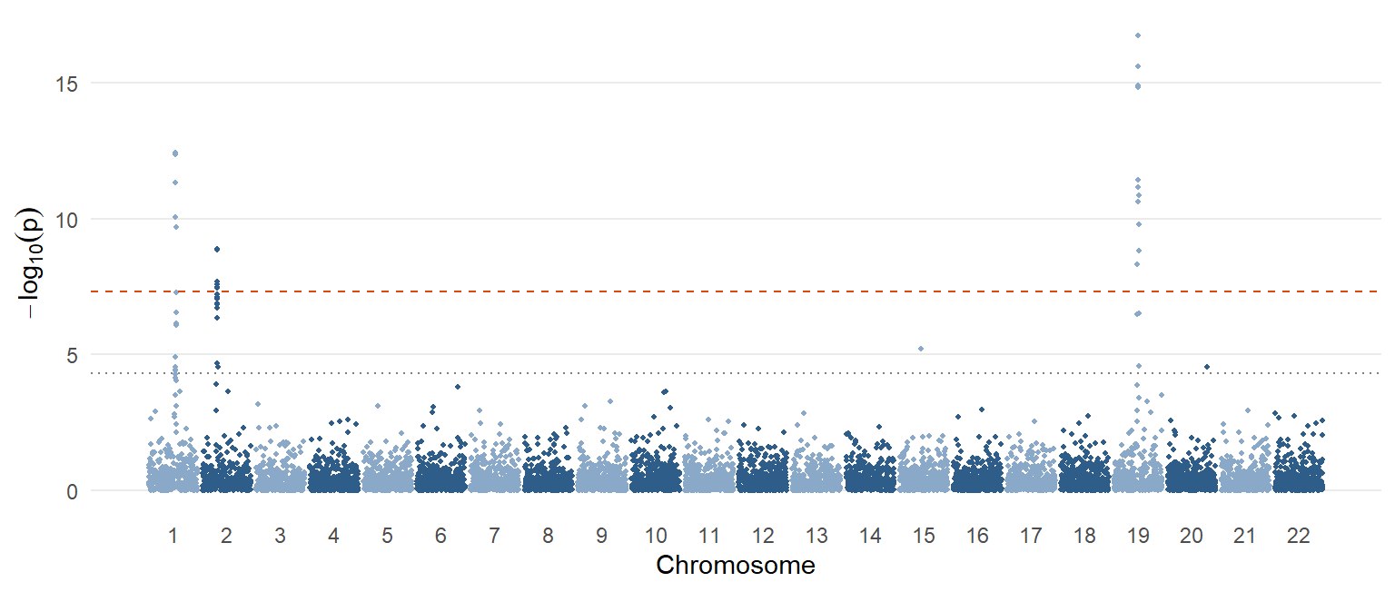
Manhattan plot. x-axis: genomic position ordered by chromosome; y-axis: \(-\log_{10}(p)\), so stronger associations are taller (“skyscrapers”). Each dot is one SNP. Horizontal lines usually mark a suggestive threshold (~5×10⁻⁵ or similar) and genome-wide significance (5×10⁻⁸).

Simulated Manhattan plot. Three loci contain a true signal; LD makes each one a tower of neighbouring SNPs rather than a single point.

Two interpretive caveats (stated explicitly in the slides)

A Manhattan plot shows where the strongest associations are. It does not tell you which variant or gene is causal.
A low p-value does not mean a large effect. With a huge sample, even a tiny effect reaches genome-wide significance.

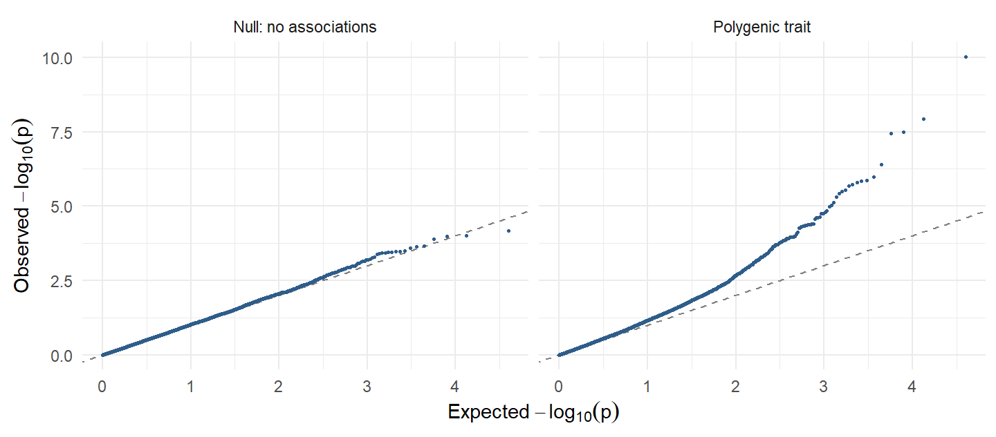
QQ plot. Observed p-values plotted against those expected under the null (no association anywhere). Points bending away from the diagonal more than chance predicts can signal a systematic problem (uncontrolled population structure, technical/batch artifacts). But it can also mean the trait is highly polygenic: very many small effects spread across the genome. That is the lecture’s explanation for LDL-C’s QQ plot looking “a bit off”: benign and expected for a polygenic trait.

Left: null SNPs follow the diagonal. Right: a polygenic trait (many small true effects) lifts the whole upper tail. Uncontrolled population structure can produce a similar lift, so the plot alone does not tell you which.

The SNP must have a large effect on the phenotype

The SNP is the causal variant at this locus

The association is statistically robust, nothing more

The SNP explains a large share of phenotype variance

A tiny p-value in a huge sample only says the association is unlikely to be chance. Effect size, causality and variance explained are separate questions (see rs11591147 in Section 4.10).

4.8 Why one signal gives a cluster: lead SNP and r²

Nearby SNPs are correlated (in LD) because they are inherited together. So one true causal variant appears as many associated SNPs: every SNP in LD with it shows an association, not because it is independently causal but because it is correlated. If two SNPs are in LD, knowing one tells you about the other. The result is one peak in the Manhattan plot.

From the cluster you pick a representative, the lead SNP: usually the one with the smallest p-value. The lead SNP is not guaranteed to be the causal variant; it may just be a good proxy.

Quantifying LD: \(r^2\), the squared correlation between two SNPs’ genotypes (0 to 1).

\(r^2\)	LD strength
> 0.8	Very strong LD; close proxy
> 0.5	Moderate to strong
< 0.1	Weak
≈ 0	Essentially independent

Downstream analyses usually need independent variables, which raises the questions of how to find independent signals and the causal variant in a correlated cluster (Lecture 5), and the complication that the causal variant might not even be measured on the array.

4.9 Population structure and confounding

The problem. If ancestry-related differences in allele frequency coincide with differences in the phenotype across subpopulations (different countries, or distinct communities such as the Amish), a SNP can look associated with the phenotype even with no biological effect at all.

	Frequency of allele G	Mean LDL-C
Population A	Higher	Higher
Population B	Lower	Lower
Pooled analysis	G looks associated with higher LDL-C, purely through the confounding, whatever G’s real effect

Standard mitigation strategies (likely asked as “how do you address population stratification in a GWAS?”):

Restrict the analysis to genetically homogeneous ancestry groups.
Adjust for genetic principal components (PC1, PC2, …).
Account for relatedness with mixed models (e.g. regenie).
Check the QQ plot and genomic inflation as a diagnostic.

Adjusting for genetic principal components

Restricting to one homogeneous ancestry group

Using mixed models that account for relatedness

Lowering the significance threshold to p < 0.05

Stratification is confounding; a different p-value threshold does not remove it. The standard tools are homogeneous samples, PC adjustment, mixed models (e.g. regenie) and QQ/inflation checks.

4.10 From hit to biology: locus, lead SNP, QTLs

Term	Definition
SNP	One specific variant
Locus	A genomic region containing one or more associated variants (often one Manhattan peak)
Lead SNP	The SNP with the smallest p-value within that locus

Worked example: rs11591147. β = −0.5 mmol/L LDL-C per T allele, a very strong effect. Allele frequency of T is only 1.5%.

Genotype	Mean LDL-C	Frequency (HWE)
GG	3.0 mmol/L	\(0.985^2 \approx 0.970\)
GT	≈ 2.5 mmol/L	\(2 \times 0.985 \times 0.015 \approx 0.03\) (3%)
TT	≈ 2.0 mmol/L	\(0.015^2 = 0.000225\) (0.023%)

Lesson: a variant can have a large per-allele effect yet explain very little population-level variance because it is rare. Effect size and population relevance are different things; consider both.

Quantitative trait locus (QTL): a genomic region where genetic variation is associated with variation in a quantitative trait. More broadly, QTL analysis asks whether a variant can be linked to any measurable molecular trait: gene expression, protein level, metabolite level.

Protein QTL (pQTL): is the SNP near the gene encoding the protein (cis-pQTL) or elsewhere in the genome (trans-pQTL)? Developed in Lecture 8 (Section 8.9).

GWAS gives associations, not yet causality

GWAS gives you: a variant–phenotype association, an effect size, a p-value and a locus.

GWAS does not tell you: which SNP in the locus is causal, which gene is causal, which pathway is involved, or whether changing the molecular trait would change disease risk.

GWAS is a discovery tool. Causal inference needs extra assumptions and methods: Mendelian randomization (Lecture 6).

Practice

Redo the worked calculations with your own numbers

Runs in your browser. Change the inputs and rerun.

Tasks

Set maf <- 0.015 (rs11591147). What share of the population are heterozygotes and minor homozygotes?
Keep maf <- 0.10 but set risk_ratio <- 1.2. How much of the case enrichment is left?
A GWAS reports OR = 1.30 per allele. What is β? What OR do you expect for two copies?

Model answer

het ≈ 0.0296 (3%), alt_hom = 0.000225 (0.023%).
The risks become 5%, 6% and 7.2%, and the shares of cases become about 78%, 21% and 1.4%, barely different from the population shares (81%, 18%, 1%). Smaller effects give smaller case–control differences, so you need larger samples to detect them.
log(1.30) ≈ 0.262. Two copies: exp(2 * log(1.30)) = 1.30² = 1.69.

Why-questions

Why is 5×10⁻⁸ the genome-wide threshold?

It is roughly 0.05 / 1,000,000: a Bonferroni correction for about a million independent common-variant tests across the genome. With p < 0.05 you would expect ~50,000 false positives.

Why do GWAS use the additive model?

It is the simplest, most tractable model that works reasonably across a million tests. Dominant or recessive models make sense when you study one gene in depth. “Dominant” is a property of the genotype–phenotype relationship, not of the allele.

Why can a highly significant SNP matter little for public health?

Significance depends on sample size. A rare variant (like rs11591147, 1.5%) can have a big per-allele effect but affect few people; a common variant with a tiny effect can be extremely significant in a million-person GWAS yet barely change anyone’s risk.

Why does a QQ plot that lifts off the diagonal not always mean a problem?

Both confounding (population structure, batch effects) and genuine polygenicity inflate many test statistics. For a highly polygenic trait like LDL-C, the lift is expected.

Spaced review

The physical distance between two genes in base pairs

Non-random association of alleles at different loci

The chance that a gamete carries a dominant allele

The frequency of recombination during mitosis

LD is the non-random association of alleles at different loci in a population, detected by comparing observed with expected haplotype frequencies.

A position that depends on the genome build used

A reference transcript version in NCBI RefSeq

A stable variant identifier in the dbSNP database

A protein sequence in the NP_ reference series

rs numbers are dbSNP identifiers and do not change between builds, unlike genomic coordinates (GRCh37 vs GRCh38).