flowchart TD
  A["High dimensionality<br/>(many features, few samples)"] --> B["Noisy measurements<br/>(technical noise,<br/>unstable variances)"]
  B --> C["Multiple testing<br/>(many tests, many false hits)"]
Lecture 7 — High-Dimensional Molecular Data
The siNET miRNA case study · technical noise and preprocessing · moderated t (limma) · log₂FC · FWER vs FDR · Bonferroni · Benjamini–Hochberg · clustering and circular reasoning
ImportantThis is the only lecture with instructor EXAM tags
The course’s reading guide says: “The slides with information that we will be testing on the exam are marked with a small text ‘EXAM.’” Every section below with the 🎯 Instructor-flagged EXAM badge carried that marker. Treat these as the highest-confidence exam content in the course. The instructor also posted “Lecture 7 - questions.pdf” with example exam questions. All 11 are on the Exam practice page with model answers.
Up to now, each analysis tested one thing: one SNP, one exposure. Omics data flips that around. You measure hundreds or thousands of molecules (here 955 microRNAs) in a few dozen samples and ask which of them differ between groups. Three problems follow in a chain: high dimensionality → noisy measurements → multiple testing.
The measurements are noisy because the lab process adds its own variation, so the data must be cleaned (background correction, normalization) before any biology is compared. With few samples per feature, the ordinary t-test becomes unreliable, and the fix is to let the features borrow strength from each other (the moderated t-statistic in limma). And with 955 tests at once, about 48 will look “significant” by chance, so the significance cutoff has to change: Bonferroni controls the chance of any false positive, Benjamini–Hochberg controls the proportion of false positives among the hits.
The lecture is built around a real study: miRNA profiling of small intestinal neuroendocrine tumours (siNETs), which found tumour subtypes and a survival biomarker, miR-375.
This page follows that study from sample to result. The BH and Bonferroni calculations have worked tables, an R exercise and a drill that generates new problems. Be able to do them by hand.
NoteSources and session
Slides: “Lecture 7 part 1 PRELIMINARY.pdf” (slide date 22 Sep 2026; updated the evening before the session “with some clarification and extra explanations”).
Case study article: Arvidsson Y, Rehammar A, Bergström A, et al. miRNA profiling of small intestinal neuroendocrine tumors defines novel molecular subtypes and identifies miR-375 as a biomarker of patient survival. Modern Pathology 2018. The full text is not in the source guide.
Rough plan: Week 4, day 1. High-dimensional data (gene expression, GO, clusters), proteomics.
7.1 Why high-dimensional data is a different problem
Classical epidemiology asks one question: is exposure X associated with outcome Y? Omics-scale molecular epidemiology asks: which of hundreds or thousands of molecular features are associated with phenotype Y, all in the same analysis.
Each link has its own section below. This chain is the opening framework and also the lecture’s take-home message.
7.2 The siNET case study
Clinical background. Small intestinal neuroendocrine tumours (siNETs) are often diagnosed only after metastasis. Five-year survival is poor but highly variable and hard to predict. Biologically they are distinctive: an unusually low mutational burden and no classic recurrent driver mutations. Tumour initiation is thought to be driven by large-scale chromosomal alterations and epigenetic factors instead. (A useful contrast with AML in Lecture 3: not every cancer is a point-mutation story.)
miRNA recap (Lecture 3): short (~22 nt) non-coding RNAs acting as epigenetic/post-transcriptional regulators: they suppress translation and reduce mRNA stability. Perfect pairing is not needed, so each miRNA regulates hundreds of mRNAs. Altered miRNA expression is found in virtually all tumour types. Aberrant miRNAs act as oncomiRs (promoting cancer) or tumour suppressors, by targeting genes for proliferation, cell cycle, apoptosis, invasion and drug resistance.
Study aim: characterize the miRNA profile of siNETs, looking for clinically relevant molecular subgroups and biomarkers of tumour development and outcome.
Samples: 42 tumours from 37 patients operated for siNET, plus 6 samples of normal small intestinal mucosa.
7.3 The microarray experiment
- RNA isolation: with a commercial kit (e.g. miRNeasy, Qiagen) from fresh-frozen tumour tissue (at least 70% tumour cells) and normal mucosa.
- Labelling and hybridization: RNA is labelled with a fluorescent dye and allowed to base-pair with known probe sequences fixed on an array (Agilent).
- Scanning: a scanner reads fluorescence intensity at every spot. Intensity is a relative measure of how much of that miRNA is present; software turns the image into numbers.
- Design details: 955 probes (866 human + 89 viral miRNAs), 4–8 replicate spots per probe (to assess consistency), 48 samples (42 tumours + 6 normal).
7.4 Observed variation = biology + technical noise
\[\text{Observed signal} = \text{biological signal} + \text{technical variation (noise)}\]
Sources of technical variation in this study: RNA extraction, labelling, hybridization, scanner/detection noise and batch effects (developed further for proteomics in Lecture 8, Section 8.6; the principle applies to every high-throughput platform).
Implication: before trusting any biological comparison, remove as much technical noise as possible. That is what preprocessing does.
To remove the biological signal so only noise is left
The measured signal also contains technical variation
To turn relative intensities into absolute concentrations
Because the t-test cannot be used on log-scale values
Observed variation = biology + technical noise (extraction, labelling, hybridization, scanner, batch). Preprocessing removes technical variation so remaining differences reflect biology.
7.5 Preprocessing: background correction and normalization
The initial analysis steps, in order:
| Step | Scope | Method in this study | What it does |
|---|---|---|---|
| 1. Quality control | |||
| 2. Background correction | Within each array | normexp | Models observed intensity = true signal + background noise, with noise ~ normal and signal ~ exponential; estimates the expected true signal given the observed intensity. Gives positive corrected values (naive subtraction can give negatives) and improves reliability of low-intensity measurements |
| 3. Normalization | Between arrays | Quantile normalization | Makes the distribution of intensities identical across arrays |
| 4. Average replicate probes | Per miRNA | Mean of the 4–8 spots | One more reliable value per miRNA |
Quantile normalization, step by step
- Within each sample, rank all values from lowest to highest.
- For each rank position, compute the mean across all samples.
- Replace each value by the mean for its rank.
It keeps each sample’s internal order (the highest miRNA in a sample stays highest) but equalizes the overall distribution. Assumption: the overall expression distribution should be similar across arrays, so any large systematic difference in distribution shape is technical, not biological.
Worked example. Four miRNAs (A–D) on three arrays.
| miRNA | Array 1 | Array 2 | Array 3 |
|---|---|---|---|
| A | 5 | 4 | 3 |
| B | 2 | 1 | 4 |
| C | 3 | 3 | 6 |
| D | 4 | 2 | 8 |
Sort each array and average across ranks:
| Rank | Array 1 | Array 2 | Array 3 | Rank mean |
|---|---|---|---|---|
| 1 (lowest) | 2 | 1 | 3 | (2+1+3)/3 = 2.000 |
| 2 | 3 | 2 | 4 | (3+2+4)/3 = 3.000 |
| 3 | 4 | 3 | 6 | (4+3+6)/3 = 4.333 |
| 4 (highest) | 5 | 4 | 8 | (5+4+8)/3 = 5.667 |
Put the rank means back in each array’s original order:
| miRNA | Array 1 | Array 2 | Array 3 |
|---|---|---|---|
| A | 5.667 (rank 4) | 5.667 (rank 4) | 2.000 (rank 1) |
| B | 2.000 (rank 1) | 2.000 (rank 1) | 3.000 (rank 2) |
| C | 3.000 (rank 2) | 4.333 (rank 3) | 4.333 (rank 3) |
| D | 4.333 (rank 3) | 3.000 (rank 2) | 5.667 (rank 4) |
Each column now contains exactly {2, 3, 4.333, 5.667}: identical distributions, original within-array order kept. Array 3’s overall higher level (technical) is gone.
Every miRNA has the same value on every array
Every array has the same set of values, in its own order
The order of miRNAs within each array is reversed
Arrays keep their original means but get equal variances
All arrays share the same distribution (the rank means), but each array keeps its own ranking of miRNAs. A miRNA’s value can still differ between arrays because its rank differs.
7.6 Supervised vs unsupervised analysis
| Supervised | Unsupervised | |
|---|---|---|
| Question | Which miRNAs differ between predefined groups? | Do samples naturally form groups based on expression? |
| Labels used? | Yes (metastasis vs primary, tumour vs normal) | No |
| Method here | Differential expression testing | Hierarchical clustering |
7.7 Why the ordinary t-test fails, and the moderated t
The ordinary two-sample t-statistic
\[t = \frac{\bar x_1 - \bar x_2}{s\sqrt{\tfrac{1}{n_1} + \tfrac{1}{n_2}}}\]
where \(s^2\) is estimated separately for every gene/miRNA from only \(n_1 + n_2 - 2\) degrees of freedom: just 4 df for 3 vs 3 samples, a very typical omics size.
Three compounding problems
- \(s^2\) is very noisy: with 4 df a feature’s variance estimate is often far from its true variance.
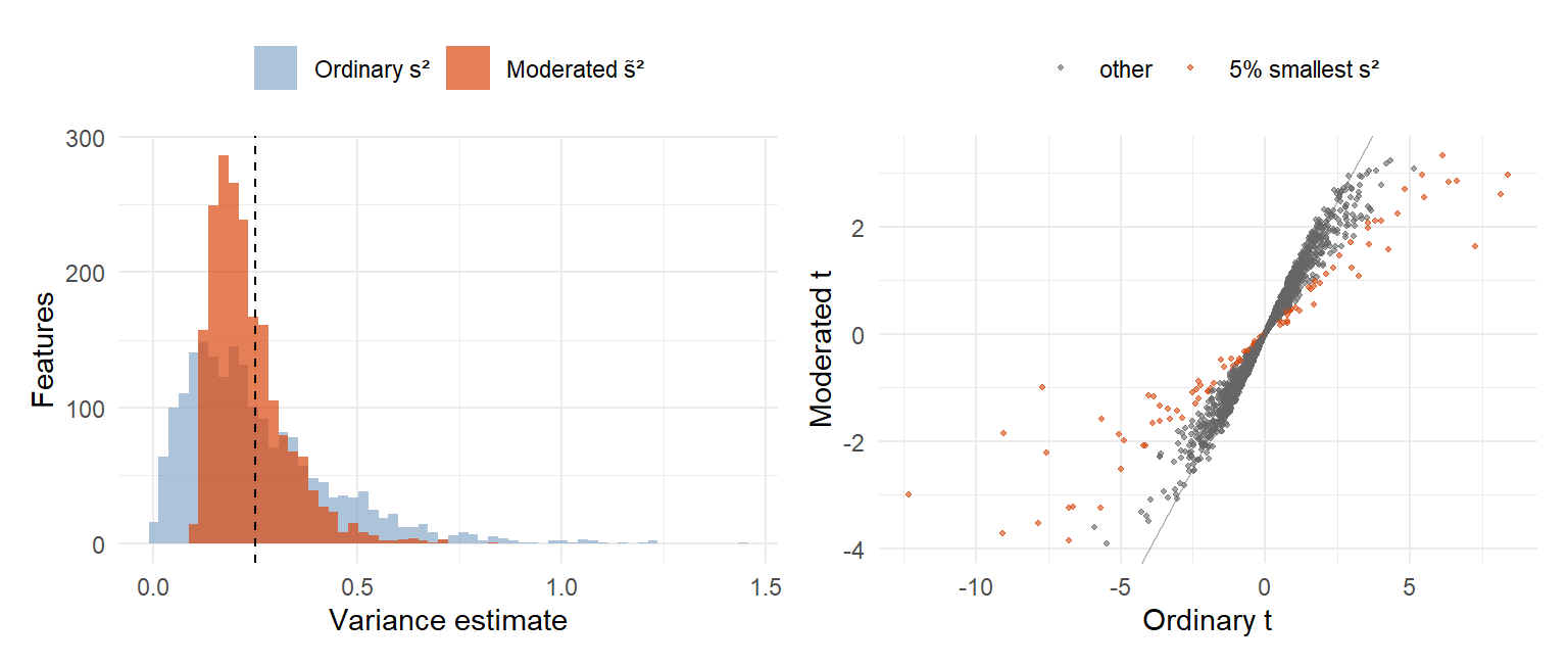
- By chance some features get a tiny \(s^2\). Since \(s^2\) is in the denominator, \(t\) becomes huge even when the mean difference is small → false positives.
- The ranking is partly driven by noise in each \(s^2\), so real effects with a larger \(s^2\) are missed → lost power.
The solution: the moderated t-statistic, R package limma. Instead of trusting each feature’s own noisy variance, limma uses empirical Bayes to share information across all features: each variance is shrunk toward a common variance estimated from the whole dataset. The result is a moderated t-statistic and p-value per feature.
The shrunken (moderated) variance is a weighted average of the common prior variance \(s_0^2\) (with prior df \(d_0\)) and the feature’s own variance \(s_g^2\) (with \(d_g\) residual df):
\[\tilde s_g^2 = \frac{d_0\, s_0^2 + d_g\, s_g^2}{d_0 + d_g}, \qquad \tilde t_g = \frac{\bar x_1 - \bar x_2}{\tilde s_g\sqrt{\tfrac{1}{n_1} + \tfrac{1}{n_2}}}\]
How shrinkage behaves (a “consequences” slide, also marked EXAM):
| Replicates | Who dominates | Effect |
|---|---|---|
| Few (small \(n_k\)) | The global weight \(d_0\) | Each variance is pulled strongly toward \(s_0^2\). This prevents false positives from randomly tiny variances |
| Many (large \(n_k\)) | The feature’s own data | The moderated variance converges to the ordinary sample variance: you trust the feature’s own estimate |
Its variance estimate is tiny by chance, inflating t
Its true biological effect is larger than all others
The array for that miRNA had too many replicate spots
The p-value was already corrected with Bonferroni
With 4 df, some variance estimates are randomly very small. A small s² in the denominator gives a huge t: a false positive. Variance shrinkage (limma) pulls it toward the common variance.
Shrinkage gets stronger, pulling every variance to s₀²
Each feature’s own variance gets more and more weight
The moderated t turns into a Bonferroni-corrected t
The prior degrees of freedom d₀ grow with the sample
With many replicates the feature’s own data dominate and the moderated variance converges to the ordinary sample variance. With few replicates the global prior (d₀) dominates.
7.8 Summary: the small-sample problem, in full
Marked EXAM across three consecutive slides. Close to a model answer for “explain why moderated statistics are needed in omics data”.
NoteModel answer structure
1. The challenge of small sample sizes. Transcriptomics, proteomics and metabolomics routinely measure tens of thousands of features on few biological replicates.
2. The failure of standard t-tests. Each feature’s variance is estimated separately from very few replicates, so the estimates are highly unstable. By chance some are abnormally low → inflated t → false positives; others abnormally high → real effects masked → lost power. Because this instability sits under every p-value, it also undermines the multiple-testing correction afterwards, which assumes well-calibrated p-values.
3. The standard solution. Sharing information across the whole dataset, known as variance shrinkage or empirical Bayes moderation, stabilizes the variance estimates: each is pulled toward a common value estimated from all features. This reduces false positives, recovers power and gives more reliable results after multiple-testing correction (e.g. FDR).
7.9 Log₂ transformation and log₂ fold change
Log₂ transformation makes expression values more symmetric and reduces the influence of very large raw values.
Log₂ fold change describes magnitude and direction of a change between groups:
| log₂FC | Fold change | Meaning |
|---|---|---|
| +3 | \(2^3 = 8\) | 8× higher |
| +2 | \(2^2 = 4\) | 4× higher |
| +1 | 2 | 2× higher |
| 0 | 1 | No change |
| −1 | 1/2 | 2× lower |
| −2 | 1/4 | 4× lower |
Power-of-2 relationship: \(\text{FC} = 2^{\log_2\text{FC}}\). The same logic returns in Lecture 8: one NPX unit (Olink/SomaScan) is a doubling.
It is 2 times lower in metastases
It is 4 times lower in metastases
It is 2 units lower on the raw intensity scale
It is 4 times higher in metastases
2^−2 = 1/4, so expression in metastases is a quarter of that in primaries: 4× lower. The sign gives the direction.
7.9b Tumour vs normal results, and the paired-sample note
Result: miR-7-5p and miR-375 were the two most significantly upregulated miRNAs in tumours vs normal mucosa. Several other differentially expressed miRNAs previously reported in the siNET literature also appeared (marked with an asterisk in the paper’s figure).
“Note… Why?” Five patients had paired samples (a primary tumour and a liver metastasis). In the tumour vs normal comparison they contributed only their primary tumour.
Why? Two samples from the same patient are not independent (same patient, same genetic background). Including both would give that patient double weight and bias variance estimates and significance tests. This is a general principle: repeated or paired samples from one subject violate the independence assumption of standard tests.
7.10 The multiple testing problem, with this study’s numbers
955 miRNAs were tested. If none truly differed, you would still expect
\[955 \times 0.05 \approx \mathbf{48}\]
“significant” hits at an uncorrected \(p < 0.05\).
The logic in three steps:
- Every test has its own 5% false-positive chance from noise alone, even for a miRNA with zero effect.
- Run hundreds or thousands of tests and those small chances accumulate: some false hits become nearly guaranteed.
- A flat \(p < 0.05\) applied test by test turns “5% error per test” into a high chance of at least one error somewhere in the study. For 955 independent null tests, \(P(\geq 1 \text{ false positive}) = 1 - 0.95^{955} \approx 1\).
Conclusion (stated directly in the slides): because this is multiple testing, the significance cutoff itself must change.
7.11 FWER vs FDR
Expect to define, distinguish and calculate both.
| FWER (Family-Wise Error Rate) | FDR (False Discovery Rate) | |
|---|---|---|
| Definition | \(P(\text{at least one false positive among all tests})\) | \(E\left[\dfrac{\text{false positives}}{\text{all positives called}}\right]\), the expected proportion of hits that are false |
| Philosophy | Even one false lead among hundreds of tests is a failure of the whole experiment: a very strict bar | Accepts a known, controlled fraction of wrong hits and controls how large that fraction is expected to be |
| Classic method | Bonferroni | Benjamini–Hochberg (BH) |
Both start from the same p-values but ask different questions, giving different, non-interchangeable cutoffs.
The chance of any false positive among the 200 is at most 5%
About 10 of the 200 hits are expected to be false positives
Each of the 200 miRNAs has a 5% chance of being a true effect
Exactly 5% of all 955 tested miRNAs are false positives
FDR = expected proportion of false positives among the hits: 5% of 200 ≈ 10. “Any false positive at most 5%” is FWER control (Bonferroni).
7.12 Bonferroni: controlling the FWER
Rule: reject \(H_0\) for test \(i\) if
\[p_i \le \frac{\alpha}{m} \qquad \text{equivalently} \qquad p_{\text{adj}} = \min(1,\; p \times m) \le \alpha\]
where \(m\) is the number of tests.
Three properties
- Valid for any \(m\), any test type, regardless of dependence between tests: no assumptions about correlation, “always safe”.
- Controls the strictest bar, the FWER: a single false positive among all tests counts as failure.
- Worked consequence for this study: \(m \approx 955\) → \(\alpha/m \approx 0.05/955 \approx \mathbf{0.00005}\). Many true effects do not survive this, so power collapses when \(m\) is large, which is typical for omics.
7.13 Benjamini–Hochberg: controlling the FDR
The BH algorithm, three steps (reproduce exactly):
- Sort the \(m\) p-values: \(p_{(1)} \le p_{(2)} \le \dots \le p_{(m)}\).
- Find the largest rank \(k\) with \(p_{(k)} \le \dfrac{k}{m}\,Q\), where \(Q\) is the accepted FDR (commonly 0.05).
- Call every test with \(p \le p_{(k)}\) significant. The expected FDR of this set is \(\le Q\).
Key difference from Bonferroni: Bonferroni has one fixed threshold \(\alpha/m\). BH’s threshold \(\frac{k}{m}Q\) rises with rank, so larger p-values can still be significant if they clear the higher bar for their rank. That is why BH finds more true positives.
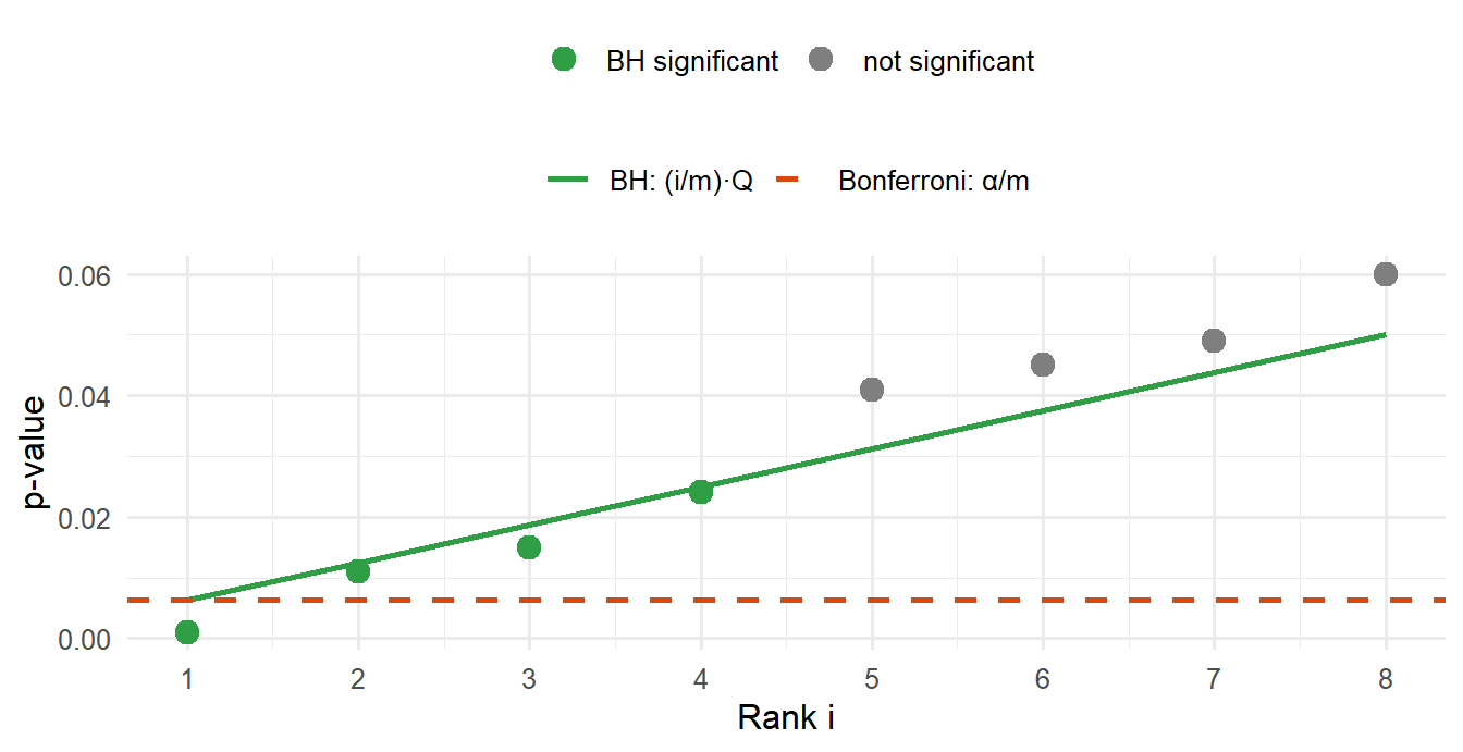
🎯 Instructor-flagged worked example: m = 8, Q = 0.05
| Rank \(i\) | \(p_{(i)}\) | Threshold \(\frac{i}{m}Q\) | \(p_{(i)} \le\) threshold? | Significant? |
|---|---|---|---|---|
| 1 | 0.001 | 0.00625 | yes | ✓ |
| 2 | 0.011 | 0.01250 | yes | ✓ |
| 3 | 0.015 | 0.01875 | yes | ✓ |
| 4 | 0.024 | 0.02500 | yes | ✓ |
| 5 | 0.041 | 0.03125 | no | — |
| 6 | 0.045 | 0.03750 | no | — |
| 7 | 0.049 | 0.04375 | no | — |
| 8 | 0.060 | 0.05000 | no | — |
Largest \(k\) with \(p_{(k)} \le\) threshold: \(k = 4\) → tests 1–4 significant.
Bonferroni on the same data: \(\alpha/m = 0.05/8 = 0.00625\) → only test 1 significant.
WarningThe “largest k” trap
BH does not stop at the first p-value that fails. You look for the largest rank that passes. If rank 5 failed but rank 6 passed, then all of ranks 1–6 would be significant, including rank 5. (In the example above no rank after 4 passes, so k = 4.)
1
2
3
4
Sort: 0.004, 0.026, 0.030, 0.045, 0.300. Thresholds (i/5)·0.05: 0.01, 0.02, 0.03, 0.04, 0.05. Rank 1 passes, rank 2 fails (0.026 > 0.02), rank 3 passes (0.030 ≤ 0.03), ranks 4 and 5 fail. The largest passing rank is k = 3, so the three smallest p-values are significant, including 0.026, which failed its own threshold. Stopping at the first failure (answer 1) is the classic mistake.
7.13b BH-adjusted p-values
BH can also be written as an adjusted p-value per test:
\[p^{\text{adj}}_{(i)} = \min_{j \ge i}\left( p_{(j)} \cdot \frac{m}{j} \right)\]
Take the smallest value of \(p_{(j)} \cdot m/j\) over all ranks from \(i\) down to the bottom of the list. This “running minimum from the bottom” makes the adjusted p-values non-decreasing down the sorted list, which \(p_{(i)} \cdot m/i\) alone does not guarantee.
🎯 Instructor-flagged worked example, same 8 tests
| Rank \(i\) | \(p_{(i)}\) | \(p_{(i)} \cdot m/i\) | Adjusted p | Significant (\(\le 0.05\))? |
|---|---|---|---|---|
| 1 | 0.001 | 0.008 | 0.008 | ✓ |
| 2 | 0.011 | 0.044 | 0.040 | ✓ |
| 3 | 0.015 | 0.040 | 0.040 | ✓ |
| 4 | 0.024 | 0.048 | 0.048 | ✓ |
| 5 | 0.041 | 0.066 | 0.056 | — |
| 6 | 0.045 | 0.060 | 0.056 | — |
| 7 | 0.049 | 0.056 | 0.056 | — |
| 8 | 0.060 | 0.060 | 0.060 | — |
How to fill the “Adjusted p” column: start at the bottom (rank 8: 0.060). Move up; each value is the minimum of its own \(p \cdot m/i\) and the adjusted value below it. Rank 7: min(0.056, 0.060) = 0.056. Rank 6: min(0.060, 0.056) = 0.056. Rank 5: min(0.066, 0.056) = 0.056. Rank 4: min(0.048, 0.056) = 0.048. Rank 3: min(0.040, 0.048) = 0.040. Rank 2: min(0.044, 0.040) = 0.040. Rank 1: min(0.008, 0.040) = 0.008.
Same decision as the threshold version (tests 1–4), but now each test has its own adjusted p-value: the format reported in most papers, including the siNET paper. In R: p.adjust(p, method = "BH").
7.14 Why FDR fits omics data
Four reasons, a strong essay-question candidate (“why is FDR preferred over Bonferroni in omics?”):
- Too many tests for Bonferroni. Thousands of tests push α/m toward zero, so most true effects never reach it.
- Exploratory, not confirmatory. The goal is a shortlist of candidates, not one make-or-break claim. A small, controlled fraction of false leads is an acceptable price for finding more true positives.
- Findings are validated afterwards with an independent method and/or cohort. The siNET study did exactly this: miR-375 was confirmed with qRT-PCR and in situ hybridization in a separate cohort.
- Features are correlated. Co-regulated miRNAs (genes, proteins) mean the effective number of independent tests is smaller than \(m\). Bonferroni ignores this and stays needlessly strict; BH copes better in practice.
Thousands of tests make Bonferroni’s threshold too strict
Screens are exploratory, and hits are validated afterwards
Correlated features make the effective number of tests smaller
FDR guarantees that no false positives are among the hits
FDR accepts a controlled proportion of false positives; it never guarantees zero. Even FWER control only bounds the probability of any false positive.
7.15 Multiple testing in the siNET paper
Quote from the methods: “All P-values were adjusted for multiple testing using Benjamini–Hochberg false discovery rate.”
| Tumour vs normal | |
|---|---|
| miRNAs tested | 955 |
| Significant (adjusted P < 0.05) | 155 (75 up, 80 down) |
| miR-375 adjusted P | 4.2 × 10⁻¹⁹ |
7.16 Cluster analysis and downstream findings
Unsupervised hierarchical clustering of miRNA profiles with complete linkage and Euclidean distance. Associations between clusters and clinical variables were tested with Fisher’s exact test and the t-test. Samples separated into normal (N), primary (P) and metastatic (M) groups; metastases split further into M1 and M2.
M1 vs M2
| Feature over-represented in M1 | P |
|---|---|
| Higher grade (G2/G3), i.e. higher proliferation | 0.0011 |
| Ki67 index > 3% (proliferation) | 0.00023 |
| Gain of chromosome 14 | 0.0013 |
(Chromosome 14 gain ties back to siNETs being driven by chromosomal alterations, Section 7.2.)
Differential expression M1 vs M2: 76 miRNAs up and 65 down in M1 (adjusted P < 0.05). Most upregulated in M1: miR-1246 and miR-663a, highly expressed in several cancers and implicated as oncomiRs (proliferation, invasiveness, metastasis). Most downregulated: miR-488-3p, reported as a tumour suppressor in gastric cancer.
Survival by cluster: patients with M1 tumours had shorter overall survival than M2 (log-rank P = 0.029; from the instructor’s example questions).
Survival analysis per miRNA: one Cox regression per miRNA, adjusted for age and gender. miR-375 was the top candidate: higher expression → longer survival. miR-375 was also shown to be expressed in liver metastases via tissue microarray.
7.16b Circular reasoning: testing clusters with the data that built them
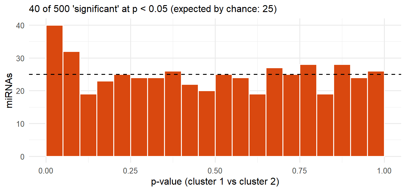
The M1/M2 clusters were created from miRNA expression (unsupervised clustering), and then miRNA expression was tested again for differences between those same clusters. The same data is used twice: once to define the groups, again to test them.
This is circular reasoning and inflates significance. Any clustering produces groups that differ in the variables used to build it, almost by construction, so “finding” that they differ is not independent evidence.
ImportantGeneral principle
Do not use one dataset to both discover a grouping and test for differences across that grouping without independent validation (a new cohort) or a correction for the selection.
The Cox regression was not adjusted for age and gender
Hierarchical clustering cannot use Euclidean distance
M1 and M2 were defined from the same miRNA data
Benjamini–Hochberg is too liberal for 955 miRNAs
The clusters were built from the expression data, so they differ in that data almost by construction. Testing the same data between those clusters is circular and inflates significance.
7.17 Take-home message
The lecture’s own closing slide:
- High dimensionality → noisy measurements → multiple testing (7.1).
- Observed variation = biological + technical variation, requiring preprocessing; quantile normalization as the worked example (7.4–7.5).
- The ordinary t-statistic fails at small sample sizes; the moderated t-statistic is the solution (7.7).
- Multiple testing: FWER vs FDR, and being able to calculate Bonferroni- and BH-adjusted values (7.10–7.13).
- Validation in an independent cohort with an independent method before treating a screening hit as established (7.14).
NoteConsolidated list of all 🎯 EXAM topics in Lecture 7
- Observed variation = biology + technical noise
- Preprocessing: QC → background correction (normexp) → normalization (quantile) → averaging replicates
- Why the ordinary t-test fails at small sample sizes
- Moderated t / limma / empirical Bayes shrinkage; behaviour at small vs large sample sizes
- The three-part summary: challenge of small samples / failure of standard t-tests / standard solution
- Log₂ transformation and log₂ fold change
- The multiple testing problem (955 × 0.05 ≈ 48)
- FWER vs FDR
- Bonferroni and its consequence (0.05/955 ≈ 0.00005)
- BH, threshold version and adjusted p-values, with worked tables
- Four reasons FDR fits omics
- Circular reasoning when testing clusters built from the same data
Practice
NoteBenjamini–Hochberg and Bonferroni: generated problems
Each click on New problem draws new p-values. Do it on paper first, then type your answers and press Check. The solution shows the full sorted table with thresholds and adjusted p-values.
NoteBH, Bonferroni and the moderated t in R
Runs in your browser (the first run takes a few seconds while R loads).
Tasks
- Change the 5th p-value to
0.030. What is \(k\) now, and which tests are significant? - Now set
p <- c(0.002, 0.020, 0.013, 0.030, 0.200)(unsorted on purpose). Work out BH on paper first, then check. - With 955 tests, what is the Bonferroni threshold? Compute
0.05 / 955. - Simulate 955 null tests:
p <- runif(955). How many have \(p < 0.05\)? How many survive BH and Bonferroni?
TipModel answer
- Sorted: 0.001, 0.011, 0.015, 0.024, 0.030, 0.045, 0.049, 0.060. Thresholds: 0.00625, 0.0125, 0.01875, 0.025, 0.03125, 0.0375, 0.04375, 0.05. Rank 5 now passes (0.030 ≤ 0.03125), later ranks fail → k = 5, tests 1–5 significant.
- Sorted: 0.002, 0.013, 0.020, 0.030, 0.200; thresholds 0.01, 0.02, 0.03, 0.04, 0.05. Ranks 1–4 all pass, rank 5 fails → k = 4. Bonferroni (0.01): only 0.002.
- 0.05/955 ≈ 5.2 × 10⁻⁵ (≈ 0.00005).
- About 48 have p < 0.05 (955 × 0.05); typically 0 survive BH or Bonferroni, as they should when nothing is real.
Tasks
- Look at the five features with the smallest \(s^2\). What happens to their t-values after moderation?
- Increase
nto 20 and rerun. Does moderation still change much? Why?
TipModel answer
- Their tiny variances are pulled up toward \(s_0^2\), so their inflated ordinary t-values shrink to ordinary sizes. Moderation removes these chance “hits”.
- With
n = 20, d = 38 dominates d₀ = 4, so \(\tilde s^2 \approx s^2\) and the two t-statistics nearly agree. Shrinkage matters most when samples are few.
Why-questions
TipWhy does BH find more hits than Bonferroni on the same data?
Bonferroni applies the same strict threshold α/m to every test. BH’s threshold (i/m)·Q grows with rank, and it controls a weaker error rate (the expected proportion of false hits, not the chance of any false hit).
TipWhy is quantile normalization justified?
It assumes that the overall distribution of expression should be about the same in every sample, so systematic differences in distribution are technical. If that assumption fails (e.g. a global biological shift in expression), quantile normalization would remove real biology.
TipWhy is the moderated t more powerful, not just more conservative?
Shrinkage also pulls randomly large variances down toward the common value, so real effects that were masked by an unlucky high s² can now be detected. And the moderated t has more degrees of freedom (d + d₀).
TipWhy was only the primary tumour used from paired patients?
A primary tumour and its metastasis come from the same patient and are not independent. Using both would double-count that patient and bias the variance estimates and tests.
TipWhy is a significant difference between clusters not a finding?
The clusters were built to be different in exactly those miRNAs. The difference is guaranteed by the method, not discovered in the data. Pure noise gives the same “result” (see the histogram in 7.16b).
Spaced review
Benjamini–Hochberg at 5% FDR
Bonferroni for about 1 million tests
A moderated t-test with shrinkage
Quantile normalization of p-values
0.05 / 1,000,000 = 5 × 10⁻⁸: a Bonferroni-style correction for about one million independent SNPs.
miRNAs match their target perfectly and silence one gene
miRNAs bind imperfectly and regulate many mRNAs
miRNAs come from double-stranded RNA made in the lab
miRNAs are translated into small regulatory proteins
miRNA binds imperfectly, so one miRNA regulates many targets; siRNA binds near-perfectly and silences one.
Further reading
The course’s reading guide summarizes the lecture’s main themes (last slide, page 51): noisy data due to technical variation, which needs quality control and preprocessing; high dimensionality with few samples, where the moderated t-statistic replaces the ordinary t; and multiple testing, FWER and FDR, Bonferroni and Benjamini–Hochberg. “The slides with information that we will be testing on the exam are marked with a small text ‘EXAM’.”
- Arvidsson Y, Rehammar A, Bergström A, et al. miRNA profiling of small intestinal neuroendocrine tumors defines novel molecular subtypes and identifies miR-375 as a biomarker of patient survival. Modern Pathology 2018. The article the case study is built on (PDF on Canvas below).
- “Lecture 7 - questions.pdf”: all 11 questions are worked through on the Exam practice page.
NoteCourse files on Canvas (GU login required)