flowchart TD
  G["genetic variant (SNP)"] --> X["exposure"]
  X --> Y["outcome"]
Lecture 6 — From GWAS to Mendelian Randomization
Imputation and proxy SNPs · Bradford Hill · instruments and the three MR assumptions · pleiotropy · Wald ratio and IVW · weighted median and MR-Egger · interpretation
Observational studies keep finding that people with high LDL cholesterol get more heart disease, but that alone cannot prove LDL causes it: smokers might have both, or early disease might change LDL. The gold standard answer is a randomized trial. Mendelian randomization (MR) uses a trial that nature already ran: at conception, each person is randomly dealt alleles that raise or lower LDL a little.
If people who inherited LDL-raising alleles also have more heart disease, and those alleles do nothing else relevant, the most plausible explanation is that LDL itself causes heart disease. Genotype cannot be changed by the disease, so reverse causation is ruled out from the start.
The whole method stands or falls on three assumptions about the genetic instrument: it must affect the exposure (relevance), it must not share causes with the outcome (independence), and it must affect the outcome only through the exposure (exclusion restriction). Most of the lecture is about checking those assumptions, especially the last one, which horizontal pleiotropy breaks.
This page covers imputation and proxy SNPs, the Bradford Hill criteria, why genes are good instruments, confounding, the three assumptions with their named threats, vertical vs horizontal pleiotropy, the Wald ratio and IVW estimate, weighted median and MR-Egger, and how to interpret an MR result. This is the lecture that ties the course together.
NoteSources and session
Slides: “Lecture 6 from GWAS to MR.pdf”. No separate reading list.
Concepts behind computer exercise 2 (instrument selection, allele alignment, reading IVW/Egger/weighted median): see Computer exercises: concepts.
Computer exercise 2 (not in the source guide) used genotype data (all_hg38_subset.pgen/.psam/.pvar/.snplist) and a coronary artery disease summary file (CAD_Summary_filtered.txt).
Rough plan: Week 3, day 1. From GWAS to Mendelian randomisation.
6.1 Imputation and proxy SNPs
The problem. You want to know whether a specific variant (rsXY) affects a phenotype, but it was not measured in your data. Or: your data has SNPs + SBP, another dataset tested the same region against stroke, but the SNP overlap is poor: your lead SNPs are missing in the other dataset and vice versa. Dead end?
Two tools solve it, both using LD structure:
| Tool | How it works |
|---|---|
| Proxy SNP | A SNP in very strong LD (\(r^2\) close to 1) with the SNP you want. It carries essentially the same signal, so it can stand in for it |
| Imputation | Uses LD patterns plus a large external reference panel to predict the genotype at a missing SNP as a (linear) combination of the measured SNPs, e.g. \(\text{SNP}_3 = \sum_{i \in \{3,5,6,8,11\}} a_i \cdot \text{SNP}_i\) (illustrative) |
Both bridge the gap between studies (or a study and a reference panel) that did not measure exactly the same SNPs.
6.2 The Bradford Hill criteria
Classical epidemiology’s considerations for judging whether an association is likely causal (predates genetic methods). Nine criteria, likely a list-recall item:
| # | Criterion | Short meaning |
|---|---|---|
| 1 | Strength | Strong associations are less likely to be fully explained by bias |
| 2 | Consistency | Repeated in different populations and studies |
| 3 | Specificity | One exposure linked to one outcome |
| 4 | Temporality | Exposure comes before outcome (the only strictly necessary one) |
| 5 | Biological gradient | Dose–response |
| 6 | Plausibility | A biologically plausible mechanism |
| 7 | Coherence | Fits with what is known about the disease |
| 8 | Experiment | Experimental change in exposure changes the outcome |
| 9 | Analogy | Similar exposures cause similar effects |
Memory aid: S-C-S-T-B-P-C-E-A, “Strong Consistent Specific Timing, Biological Plausible Coherent Experimental Analogy”.
6.3 Genetic variants as instruments
Key insight: genetic variants are natural instrumental variables. Genotype is fixed at conception, so it comes first in any causal chain: no reverse causation (adult disease cannot change the genotype you were born with).
To use a SNP to study the causal effect of an exposure on an outcome, three core assumptions must hold: relevance, independence, exclusion restriction (Section 6.5 gives them in full).
6.4 Why we need MR: confounding
Motivating problem. Does LDL-C cause coronary heart disease (CHD)? Observationally, high LDL-C precedes CHD, but how do you rule out:
- confounding, e.g. smoking affects both:
LDL-C ← SMOKING → CHD - selection bias
- measurement error
- reverse causation (which came first?)
The classical gold standard is the randomized controlled trial (RCT): intervene on LDL-C and see whether CHD risk changes. RCTs are expensive, slow, and not always ethical or feasible.
The genetic parallel. A naturally occurring SNP that raises or lowers LDL-C is allocated at random at conception, because meiosis randomly allocates alleles to offspring, much as an RCT randomly allocates treatment. Hence Mendelian randomization: SNP → LDL-C → CHD.
| RCT | Mendelian randomization | |
|---|---|---|
| Random allocation | Treatment assigned by researcher | Alleles assigned at meiosis |
| “Intervention” | Drug lowers LDL-C | Allele lowers LDL-C (lifelong) |
| Confounding | Balanced by randomization | Balanced, if the independence assumption holds |
| Reverse causation | Excluded by design | Excluded: genotype fixed at conception |
Why is a GWAS association with CHD not enough? It says a SNP is associated with CHD (or LDL-C), not which pathway or which gene. The SNP could act through LDL-C, or through inflammation or blood pressure (SBP). MR is designed to resolve this.
6.5 Instruments and the three MR assumptions
Selecting instruments. Choose SNPs strongly associated with the exposure (e.g. LDL-C), typically \(P < 5 \times 10^{-8}\) in the exposure GWAS, and independent of each other (low LD, e.g. \(r^2 < 0.01\), via LD clumping, Lecture 5). At this stage you do not look at the SNP → outcome relationship at all; that comes in later.
ImportantThe three MR assumptions (the most important definitional block in the course)
| # | Assumption | Meaning | Named threats |
|---|---|---|---|
| 1 | Relevance | The variant has a robust, strong association with the exposure. Usually checked by genome-wide significance in the exposure GWAS | Weak instruments bias and destabilize the estimate |
| 2 | Independence | The variant is not associated with confounders of the exposure–outcome relationship | Population stratification, assortative mating (non-random mate choice related to the trait), selection effects (participation depends on genotype and outcome) |
| 3 | Exclusion restriction | The variant affects the outcome only through the exposure | Horizontal pleiotropy: another pathway. Ask: “does this SNP affect the outcome through another pathway entirely?” |
Relevance, because the SNP is only weakly linked to LDL-C
Independence, because blood pressure confounds the SNP
Exclusion restriction, through horizontal pleiotropy
None, because this is vertical pleiotropy through LDL-C
The SNP reaches CHD through a pathway (blood pressure) that bypasses LDL-C. That is horizontal pleiotropy, which violates the exclusion restriction.
A SNP that explains very little of the exposure variance
Allele frequency and outcome both differ between ancestries
A SNP that affects the outcome through inflammation
A SNP whose effect on the exposure is in SD units
Population stratification links the SNP to confounders (ancestry-related factors), violating independence. A weak SNP is a relevance problem; an alternative pathway is an exclusion restriction problem.
6.6 Multiple instruments, dose–response and pleiotropy
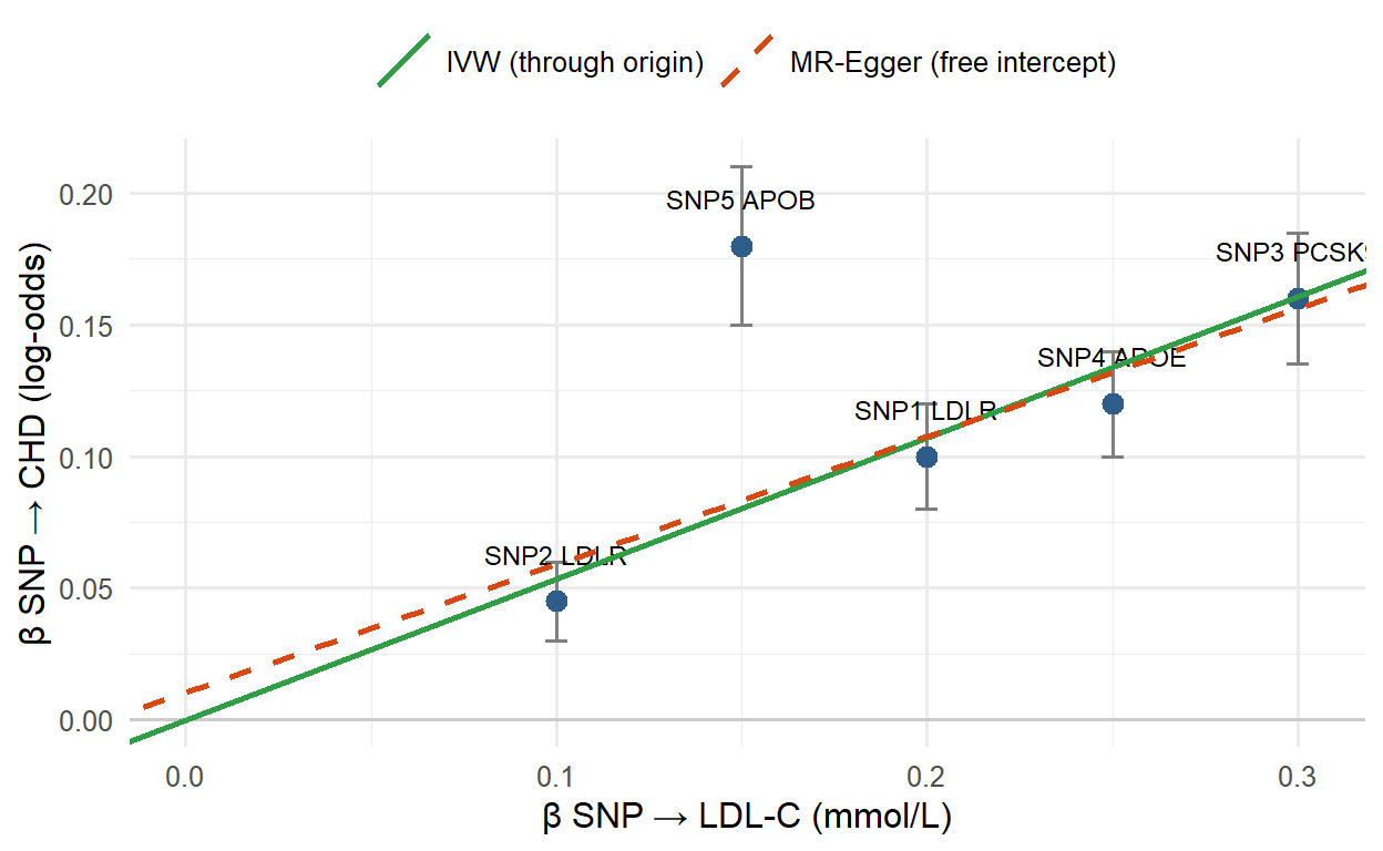
With several independent instruments, each shifting the exposure by a different amount, plot each SNP’s effect on the exposure (β-exposure, e.g. β-LDL-C) against its effect on the outcome (β-outcome, e.g. β-CHD). Example SNPs: SNP1 (LDLR), SNP2 (LDLR), SNP3 (PCSK9), SNP4 (APOE), SNP5 (APOB), all genes with known roles in LDL metabolism. A consistent dose–response line (larger effect on exposure → proportionally larger effect on outcome) strengthens confidence in causality.
Pleiotropy: one variant affecting more than one trait or pathway.
| Vertical pleiotropy | Horizontal pleiotropy | |
|---|---|---|
| Path | SNP affects the outcome via the exposure | SNP affects the outcome through a pathway independent of the exposure |
| Example | SNP1 → PCSK9 → LDLR availability → LDL-C → atherosclerosis → CHD; or SNP2 → APOE → binding → same pathway | SNP3 → LDL-C → atherosclerosis → CHD, and SNP3 → inflammation → CHD |
| For MR | Not a problem: this is the causal chain MR is looking for | Bad: violates the exclusion restriction |
6.7 The Wald ratio and IVW
One instrument: the Wald ratio
\[\hat\beta_{MR} = \frac{\beta_{\text{SNP}\to\text{outcome}}}{\beta_{\text{SNP}\to\text{exposure}}}\]
“Change in outcome per genetically predicted unit change in exposure.” If the outcome is binary, β-outcome must be on the log-odds scale. The three assumptions must still hold.
Many instruments. Compute a Wald ratio per instrument (after LD clumping), then combine. If instruments give noticeably different ratios, that disagreement is informative: horizontal pleiotropy in some instruments, or weak instruments.
Inverse-variance-weighted (IVW) MR, the standard way to combine: a linear regression of β-outcome on β-exposure across the instruments, through the origin, weighted by precision. Equivalent to a weighted average of the Wald ratios:
\[\hat\beta_{IVW} = \frac{\sum_j \beta_{X_j}\beta_{Y_j}\,/\,\sigma_{Y_j}^2}{\sum_j \beta_{X_j}^2\,/\,\sigma_{Y_j}^2}\]
where \(\beta_{X_j}\) is SNP \(j\)’s effect on the exposure, \(\beta_{Y_j}\) on the outcome, and \(\sigma_{Y_j}\) the SE of \(\beta_{Y_j}\). (The slides describe the weights as the precision of the estimates, “or a combined variance term”; the formula above is the standard first-order version.)
Outlier instruments, whose Wald ratio deviates from the rest, can arise from:
- pleiotropy / a different biological pathway
- measurement error
- a weak instrument
- population differences between the exposure and outcome studies
- chance
Agreement strengthens confidence; strong disagreement motivates sensitivity analyses.
Worked example (illustrative numbers, not from the slides). LDL-C in mmol/L, CHD on the log-odds scale.
| SNP | Gene | β exposure (LDL-C) | β outcome (log-odds CHD) | SE outcome | Wald ratio |
|---|---|---|---|---|---|
| SNP1 | LDLR | 0.20 | 0.100 | 0.020 | 0.50 |
| SNP2 | LDLR | 0.10 | 0.045 | 0.015 | 0.45 |
| SNP3 | PCSK9 | 0.30 | 0.160 | 0.025 | 0.53 |
| SNP4 | APOE | 0.25 | 0.120 | 0.020 | 0.48 |
| SNP5 | APOB | 0.15 | 0.180 | 0.030 | 1.20 (outlier) |
IVW over all five: \(\hat\beta_{IVW} \approx 0.54\) → OR ≈ \(e^{0.54} \approx 1.71\) per 1 mmol/L genetically higher LDL-C. Without SNP5: ≈ 0.50 (OR ≈ 1.65). SNP5’s much larger ratio hints at pleiotropy. Check with the Practice code below.
2.0; each allele doubles CHD risk
0.08; CHD odds rise 8% per allele
0.5; log-odds of CHD rise 0.5 per mmol/L LDL-C
0.5; half of CHD cases are caused by LDL-C
β_MR = 0.2 / 0.4 = 0.5 on the log-odds scale per 1 mmol/L genetically higher LDL-C, i.e. OR = e^0.5 ≈ 1.65 per mmol/L.
6.8 Sensitivity analyses: weighted median and MR-Egger
| IVW | Weighted median | MR-Egger | |
|---|---|---|---|
| Idea | Weighted regression through the origin = weighted mean of Wald ratios | Weighted median of the Wald ratios | Weighted regression with a free intercept |
| Valid if | All instruments valid (or pleiotropy balanced) | At least ~50% of the total instrument weight comes from valid instruments | Pleiotropic effects are independent of instrument strength (the InSIDE assumption; the slides do not use the acronym) |
| Robust to | Nothing in particular | A minority of invalid SNPs | Directional pleiotropy |
| Extra output | Non-zero intercept = signal of directional horizontal pleiotropy | ||
| Downsides | One bad instrument can distort it | Less precise, more sensitive to weak instruments, extra assumptions |
ImportantTriangulation
If IVW, weighted median and MR-Egger all point in a similar direction, confidence in causality increases substantially. The methods have different weaknesses, which are unlikely to all bias the result the same way.
The instruments are too weak to estimate anything
The exposure has no causal effect on the outcome
Directional horizontal pleiotropy among the instruments
The IVW estimate is more reliable than usual here
IVW forces the line through the origin. A non-zero Egger intercept means SNPs affect the outcome on average even with zero effect on the exposure: directional pleiotropy.
It needs only half of the instrument weight to be valid
It removes every SNP with a non-zero Egger intercept
It forces the regression line through the origin
It gives all SNPs exactly the same weight
The weighted median is consistent if at least ~50% of the weight comes from valid instruments, so a minority of invalid SNPs cannot dominate it.
6.9 Interpreting an MR result
An MR estimate is the expected change in outcome per genetically predicted change in exposure. Always check:
- The unit of exposure: per 1 SD? per 1 mmol/L? a transformed scale? Without it the magnitude is meaningless.
- Direction: \(\beta > 0\) → higher exposure increases outcome risk; \(\beta < 0\) → higher exposure decreases it.
For a binary outcome, report \(e^{\beta}\) as an OR per unit of exposure.
Practice
NoteWald ratios, IVW and MR-Egger in R
Runs in your browser. These are the numbers from the worked example in Section 6.7.
Tasks
- Which SNP has the most deviating Wald ratio? Rerun IVW without it (
mr[-5, ]). How much does the estimate change? - Look at the MR-Egger intercept with and without SNP5. What does it suggest?
- Compute a weighted median by hand: sort the Wald ratios, give each SNP weight \(\propto \beta_X^2/\sigma_Y^2\), and find where the cumulative weight passes 50%.
TipModel answer
- SNP5 (APOB): Wald ratio 1.20 vs about 0.45–0.53 for the others. IVW drops from about 0.54 to about 0.50 (OR from ≈ 1.71 to ≈ 1.65).
- The intercept is small either way (about +0.011 with SNP5 and −0.010 without) and its SE is large, so Egger cannot tell you much with only 4–5 SNPs. That is exactly its known weakness: low precision. A single outlying SNP is better picked up by comparing Wald ratios and by the weighted median.
- The 50% point falls on one of the valid SNPs (around 0.50), not on SNP5, so the weighted median barely notices the outlier.
w <- mr$bx^2 / mr$se^2
o <- order(mr$wald)
data.frame(wald = mr$wald[o], cum_weight = cumsum(w[o]) / sum(w))
Why-questions
TipWhy is MR sometimes called a “natural RCT”?
Alleles are randomly allocated at meiosis, independent of lifestyle and most confounders, just as treatment is randomly allocated in a trial. Genotype also cannot be changed by the disease, so reverse causation is excluded.
TipWhy is vertical pleiotropy fine but horizontal pleiotropy not?
Vertical pleiotropy is just the causal chain through the exposure broken into biological steps, which is exactly what MR measures. Horizontal pleiotropy adds a second route to the outcome that bypasses the exposure, so part of the SNP–outcome association is wrongly credited to the exposure.
TipWhy use several MR methods on the same data?
Each method fails under different conditions: IVW if any instrument is invalid, weighted median if more than half the weight is invalid, MR-Egger if InSIDE fails (and it is imprecise). Agreement across methods is much stronger evidence than any one estimate.
TipWhy do instruments need to be independent (clumped)?
IVW treats each SNP as a separate piece of evidence. Correlated SNPs repeat the same information, which overstates precision and can let one locus dominate.
Spaced review
Standing in for a missing SNP it is in strong LD with
Removing correlated SNPs so only one per locus remains
Testing whether the lead SNP is independent of others
Estimating ancestry principal components for adjustment
A proxy SNP has r² close to 1 with the SNP you want and carries essentially the same signal. Removing correlated SNPs is LD clumping.
Age and sex
Genotyping batch and study center
Genetic principal components
BMI and smoking status
Genetic PCs capture ancestry differences. Age and sex are biological covariates; batch and center are technical.
Further reading
No separate reading list beyond the lecture notes. The Uffelmann et al. GWAS primer (Lecture 4) is useful background for instrument selection.
- Concepts behind computer exercise 2, practised on simulated data: Computer exercises: concepts
NoteCourse files on Canvas (GU login required)