Standard linear regression rests on a critical assumption: all observations are independent. In many real datasets, this assumption is violated because observations are clustered:
Patients recruited from multiple hospitals (patients within hospitals)
Students tested in multiple schools (students within schools)
Repeated measurements on the same individual over time (measurements within individuals)
Clustered observations within the same group tend to be more similar to each other than observations from different groups, even after accounting for covariates. Ignoring this structure does not bias regression coefficients, but it underestimates standard errors, leading to false positives.
Observations within a cluster share variance, so the effective sample size is smaller than N
Clustering makes coefficient estimates biased toward the null, shrinking the apparent effect size
The residuals become skewed and non-normal, violating a key regression assumption
Clustering violates the linearity assumption, causing standard errors to shrink systematically
Within-cluster correlation means observations carry less independent information than N suggests. The effective sample size lies between m (number of groups) and N, depending on the ICC. Smaller effective N → larger true SE → OLS underestimates uncertainty.
1.2 Three approaches to clustering
Suppose we model an outcome \(Y_{ij}\) (observation \(j\) in group \(i\)) as a function of a predictor \(x_{ij}\):
No pooling — estimate a separate intercept for each group using dummy variables: \[Y_{ij} = \beta_0 + \beta_1 x_{ij} + \alpha_i + \varepsilon_{ij}, \quad \alpha_i \text{ fixed}\]
Partial pooling (mixed model) — treat group intercepts as drawn from a distribution: \[Y_{ij} = \beta_0 + \beta_1 x_{ij} + b_i + \varepsilon_{ij}, \quad b_i \sim \mathcal{N}(0, \sigma_b^2)\]
ImportantWhy partial pooling is usually best
Complete pooling ignores clustering → biased SEs
No pooling uses \(m-1\) df on nuisance parameters, gives no generalisation beyond observed groups
Partial pooling borrows strength across groups: small groups are shrunk towards the grand mean (regularisation). It generalises to unobserved groups from the same population.
Partial pooling averages the group estimate with the complete pooling estimate
Partial pooling shrinks group estimates towards the grand mean, with more shrinkage for smaller or noisier groups
Partial pooling uses only half the observations in each group
Partial pooling pools the residual variance but estimates separate intercepts without shrinkage
BLUPs (Best Linear Unbiased Predictors) are pulled towards the grand mean. The amount of shrinkage is λ = σ²_b / (σ²_b + σ²/n_i): groups with fewer observations (small n_i) or smaller between-group variance are shrunk more.
1.3 Visualising the three approaches
set.seed(7)m <-10; n <-4# many groups, few obs per group → clear shrinkageb_true <-rnorm(m, 0, 2.5)dat <-data.frame(group =factor(rep(1:m, each = n)),b_i =rep(b_true, each = n),x =rnorm(m * n, 0, 1))dat$y <-5+1.5* dat$x + dat$b_i +rnorm(m * n, 0, 3)# Fit all threefit_pool <-lm(y ~ x, data = dat)fit_nopool <-lm(y ~ x + group, data = dat)fit_mixed <-lmer(y ~ x + (1| group), data = dat)# Extract interceptsint_pool <-rep(coef(fit_pool)[1], m)int_nopool <-coef(fit_nopool)[1] +c(0, coef(fit_nopool)[3:(m+1)])int_mixed <-fixef(fit_mixed)[1] +ranef(fit_mixed)$group[,1]comp <-data.frame(group =1:m,true =5+ b_true,pool = int_pool,no_pool = int_nopool,mixed = int_mixed)cat("Group intercepts — true vs. estimated:\n")
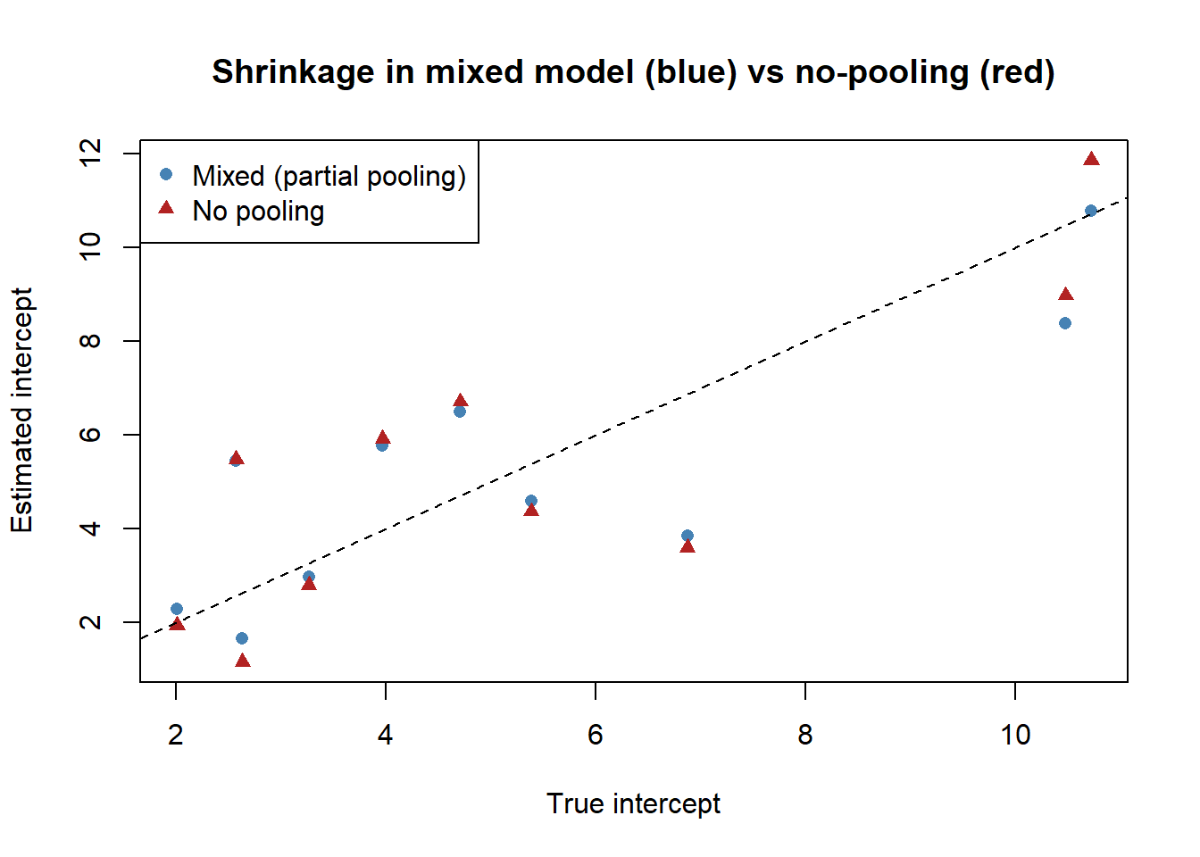
# Shrinkage: mixed model pulls estimates towards the grand meanplot(comp$true, comp$mixed, pch =16, col ="steelblue",xlab ="True intercept", ylab ="Estimated intercept",main ="Shrinkage in mixed model (blue) vs no-pooling (red)",xlim =range(comp$true),ylim =range(c(comp$mixed, comp$no_pool)))points(comp$true, comp$no_pool, pch =17, col ="firebrick")abline(0, 1, lty =2)legend("topleft", c("Mixed (partial pooling)", "No pooling"),pch =c(16, 17), col =c("steelblue", "firebrick"))
TipWhat to notice
Mixed model estimates (blue) are pulled towards the diagonal line (true values) more reliably than no-pooling (red). The shrinkage is strongest for groups with few observations or extreme raw estimates.
The complete pooling estimate (one intercept for all groups)
The no-pooling estimate for each group
The line where estimated intercept equals true intercept — perfect estimation
The grand mean intercept across all groups
The diagonal y = x marks perfect recovery of the true values. Points close to it are well-estimated. Mixed model BLUPs generally cluster closer to this line than no-pooling estimates, especially for small or extreme groups.
2 Worked Example: Multi-Centre Trial
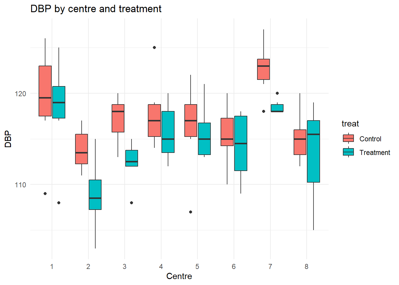
A randomised trial recruits patients from 8 hospitals. Each patient gets either treatment or control. We compare DBP at end of study.
set.seed(42)n_c <-8; n_p <-12b <-rnorm(n_c, 0, 3.5)dat_trial <-data.frame(center =factor(rep(1:n_c, each = n_p)),b_i =rep(b, each = n_p),treat =factor(rep(c(0,1), n_c * n_p /2), labels =c("Control","Treatment")),dbp1 =round(rnorm(n_c * n_p, 90, 8)))dat_trial$dbp <-round(80+ (-3)*as.numeric(dat_trial$treat=="Treatment") +0.4*dat_trial$dbp1 + dat_trial$b_i +rnorm(n_c*n_p, 0, 2))ggplot(dat_trial, aes(x = center, y = dbp, fill = treat)) +geom_boxplot() +labs(title ="DBP by centre and treatment",x ="Centre", y ="DBP") +theme_minimal()
               Estimate Std. Error t value
(Intercept)     82.8830     2.1997 37.6785
treatTreatment  -2.9125     0.3716 -7.8374
dbp1             0.3818     0.0222 17.2158
Notice: the treatment SE is larger in the mixed model. The OLS SE is anti-conservative because it treats 96 patients as 96 independent data points, ignoring that patients within the same centre share an unmeasured environment.
The mixed model estimates extra variance components that inflate uncertainty for every fixed effect regardless of the predictor's level
OLS is more efficient than the mixed model because it avoids estimating variance components and uses all N patients as independent
Treatment is assigned at the centre level — only m = 8 centres are independent; OLS treats all 96 patients as independent instead
dbp1 has the same SE in both models, which shows the inflated treatment SE in the mixed model must be a computational artefact
Note that dbp1 has the same SE in both models (0.08) — it varies patient-by-patient within centres, so all 96 observations contribute independent information. Treatment, however, is a between-centre predictor: every patient in a centre gets the same assignment. The true independent units for the treatment comparison are the 8 centres. OLS divides by √96 ≈ 9.8; the mixed model recognises only ~8 effective units. SE ratio ≈ 9.8/2.8 ≈ 3.5, consistent with the output (2.13/0.45 ≈ 4.7). The OLS p-value of 0.000 is a false positive.
3 Guided Practice
R is loading in the background — the exercises below will be interactive once the status bar disappears. You can read the concept sections above immediately.
R is loading in the background — the exercises below will be interactive once the status bar disappears. You can read the concept sections above immediately.
TipHints
Random intercept for school: (1 | school)
The SE discrepancy direction depends on the ICC — compute it from VarCorr(fit_school) to understand why
4 Retrieval Challenge
NoteModel answer
The OLS model assumes all 200 observations are independent. But each patient contributes 4 measurements — these are correlated within patient. The correct model is a random intercept (or random slope) model:
lmer(pain ~ time + treatment + (1| patient), data = d_pain)
5 Why-Questions
CautionQ: “I have only 5 groups. Is it worth using a mixed model?”
With very few groups (< 5–6), estimating \(\sigma_b^2\) is unreliable — the variance component is based on only a few observations of the random effect. In this case, a fixed effects model (no-pooling) may actually be preferable, even though it is less elegant.
Rule of thumb: mixed models become clearly beneficial with ≥ 6–8 groups, and are most powerful with ≥ 20 groups. With 5 groups, use a mixed model but report the variance component uncertainty honestly, or consider a Bayesian approach with an informative prior on \(\sigma_b^2\).
CautionQ: “Can I test whether the random intercept is needed at all?”
Yes — compare the mixed model to OLS using a likelihood ratio test. But be careful: the null hypothesis \(H_0: \sigma_b^2 = 0\) is on the boundary of the parameter space (variances can’t be negative). The standard \(\chi^2_1\) distribution is anti-conservative; the correct null distribution is a 50:50 mixture of \(\chi^2_0\) and \(\chi^2_1\).
In practice, if there is a known clustering structure in the design, include the random effect regardless of the test result — it is a design feature, not a data-driven choice.
fit_rev <-lm(y_rev ~ x_rev)coef(fit_rev) # should be close to (2, 3)
NoteFurther reading
Brown, H. & Prescott, R. (2015). Applied Mixed Models in Medicine (3rd ed.). Wiley. Companion datasets and code: wiley.com/go/brown/applied_mixed. — Chapters 1 and 2 (excluding section 2.3).