CS2.1 — From Binary to Polytomous Outcomes

1 Concept: Categorical Outcomes with More Than Two Levels

1.1 Why logistic regression is not enough

Binary logistic regression models a single log-odds:

\[\log \frac{P(Y=1)}{P(Y=0)} = \mathbf{x}^\top \boldsymbol{\beta}\]

When \(Y\) has \(K > 2\) unordered levels (e.g., disease type, treatment choice, impairment category), a single equation is insufficient. We need to model the probability of each category simultaneously.

When the outcome has exactly two categories but one is rare

When the outcome has three or more unordered categories

When the outcome is continuous and skewed

When the predictors are correlated with each other

Binary logistic regression models a single log-odds for a two-category outcome. With K > 2 unordered categories, we need K−1 simultaneous equations — one for each non-reference category. Multinomial regression generalises binary logistic regression to this setting.

1.2 The multinomial distribution

For a categorical outcome \(Y \in \{1, 2, \ldots, K\}\), the response for observation \(i\) follows a multinomial distribution with probabilities \(\pi_{ik} = P(Y_i = k | \mathbf{x}_i)\), where:

\[\sum_{k=1}^{K} \pi_{ik} = 1 \quad \forall i\]

1.3 The baseline-category logit model

Choose one category \(r\) as the reference (baseline). The model specifies \(K-1\) simultaneous logistic equations:

\[\log \frac{\pi_{ik}}{\pi_{ir}} = \mathbf{x}_i^\top \boldsymbol{\beta}_k, \quad k \neq r\]

Each equation has its own coefficient vector \(\boldsymbol{\beta}_k\) — the effect of a predictor can differ across categories.

The probabilities are recovered via the softmax transformation:

\[\pi_{ik} = \frac{\exp(\mathbf{x}_i^\top \boldsymbol{\beta}_k)}{1 + \sum_{j \neq r} \exp(\mathbf{x}_i^\top \boldsymbol{\beta}_j)}, \quad \pi_{ir} = \frac{1}{1 + \sum_{j \neq r} \exp(\mathbf{x}_i^\top \boldsymbol{\beta}_j)}\]

Key properties

With \(K\) categories, there are \(K-1\) equations, each with \(p\) coefficients → \((K-1) \times p\) parameters total
The choice of reference category does not affect predicted probabilities — only the sign/interpretation of coefficients changes
The log-OR between any two non-reference categories can be derived by subtraction: \(\log(\pi_{ik}/\pi_{ij}) = \mathbf{x}^\top(\boldsymbol{\beta}_k - \boldsymbol{\beta}_j)\)

The relative probability of being impaired versus being in any other outcome category

The change in log-odds of being impaired vs well for a one-unit increase in the predictor

The change in log-odds of being impaired relative to the mean outcome category log-odds

The predicted probability of belonging to the impaired category for a given predictor value

The baseline-category model specifies log(π_k / π_r) = x'β_k for each non-reference category k. The coefficient β_kj is the log-odds ratio for category k vs the reference r, per unit increase in predictor j. Each non-reference category has its own coefficient vector.

1.4 Why not fit \(K-1\) separate binary logistic regressions?

Fitting separate binaries (e.g., well vs rest, mild vs rest) ignores the constraint \(\sum \pi_k = 1\). Predicted probabilities may not sum to 1, and the equations are estimated independently when they should be estimated jointly. The multinomial model is the correct, joint approach.

4 — one per category

3 — one for each non-reference category

6 — one for each pair of categories

1 — the model collapses to a single log-odds

The model estimates K−1 = 3 equations, each comparing one category to the reference. The reference category's probabilities are determined by the constraint that all probabilities sum to 1. With p predictors and K=4, the model has (K−1)×(p+1) = 3(p+1) parameters.

1.5 Visualising the model structure

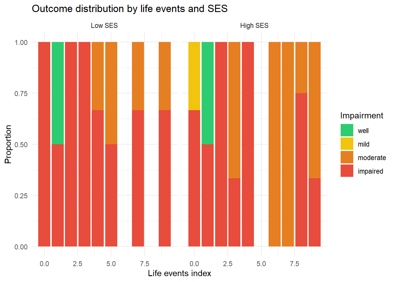
ggplot(dat, aes(x=life, fill=impair)) +
  geom_bar(position="fill") +
  facet_wrap(~ses, labeller=labeller(ses=c("0"="Low SES","1"="High SES"))) +
  labs(title="Outcome distribution by life events and SES",
       x="Life events index", y="Proportion", fill="Impairment") +
  scale_fill_manual(values=c("well"="#2ecc71","mild"="#f1c40f",
                             "moderate"="#e67e22","impaired"="#e74c3c")) +
  theme_minimal()

What to notice

As life events increase, the proportion of well decreases and impaired increases. High SES (right panel) has more well at every life events level — this is what the model will quantify.

2 Worked Example: Setting Up the Model

str(dat)

'data.frame':   40 obs. of  3 variables:
 $ ses   : num  1 1 1 1 1 1 1 1 1 1 ...
 $ life  : int  0 4 0 8 9 3 1 9 0 7 ...
 $ impair: Factor w/ 4 levels "well","mild",..: 4 4 4 3 4 4 4 3 2 3 ...

table(dat$impair)


    well     mild moderate impaired 
       2        1       11       26

table(dat$ses, dat$impair)

   
    well mild moderate impaired
  0    1    0        4       15
  1    1    1        7       11

library(nnet)
dat$impair <- relevel(dat$impair, ref="well")
fit <- multinom(impair ~ ses + life, data=dat, trace=FALSE)
summary(fit)

Call:
multinom(formula = impair ~ ses + life, data = dat, trace = FALSE)

Coefficients:
         (Intercept)        ses       life
mild      -9.6524830 10.2207398 -9.5612665
moderate  -2.0862116  0.9792450  1.1308230
impaired   0.5977727  0.1908853  0.8651376

Std. Errors:
         (Intercept)        ses        life
mild      213.966497 213.970763 170.7992513
moderate    1.708396   1.766166   0.6480470
impaired    1.447733   1.630854   0.6337955

Residual Deviance: 54.68276 
AIC: 72.68276

The output shows: - Coefficients: one row per non-reference category, one column per predictor - Std. Errors: used for Wald tests and CIs - Residual Deviance: \(-2\ell(\hat{\boldsymbol{\beta}})\) — lower is better fit - AIC: \(-2\ell + 2p\) — penalises complexity

# Wald z-tests: coefficient / SE
z <- summary(fit)$coefficients / summary(fit)$standard.errors
p <- 2 * (1 - pnorm(abs(z)))
cat("=== Z-statistics ===\n"); round(z, 3)

=== Z-statistics ===

         (Intercept)   ses   life
mild          -0.045 0.048 -0.056
moderate      -1.221 0.554  1.745
impaired       0.413 0.117  1.365

cat("\n=== P-values ===\n");     round(p, 3)


=== P-values ===

         (Intercept)   ses  life
mild           0.964 0.962 0.955
moderate       0.222 0.579 0.081
impaired       0.680 0.907 0.172

3 Guided Practice

R is loading in the background — the exercises below will be interactive once the status bar disappears. You can read the concept sections above immediately.

Hints

multinom(mode ~ distance + income, data=transport_dat, trace=FALSE)
Negative coefficient for distance in the cycle equation means…?
The reference category is car

4 Retrieval Challenge

Model answers

Q1: \((K-1) \times p = 3 \times 3 = 9\) parameters.

Q2: OR = exp(0.4) ≈ 1.49. For each one-unit increase in \(x\), the odds of mild impairment relative to being well are multiplied by 1.49 — a 49% increase.

Q3: Yes — by the log-OR subtraction property. This works because all log-ORs are relative to the same reference category, so the reference cancels.

5 Why-Questions

Q: “I changed the reference category. My coefficients all changed — did the model change?”

No — the predicted probabilities \(\hat{\pi}_{ik}\) are invariant to the choice of reference. Only the parameterisation changes. Changing the reference is like translating the coordinate system.

If you need the OR for category \(j\) vs category \(k\) (neither being the reference), compute it as: \(\exp(\hat{\beta}_{jl} - \hat{\beta}_{kl})\) for predictor \(l\), as shown in the retrieval challenge.

Q: “The outcome has an ordering: well < mild < moderate < impaired. Should I use multinomial regression?”

Not necessarily. If the ordering is meaningful, a cumulative link model (CS3) is more parsimonious — it uses a single slope per predictor instead of \(K-1\). The multinomial model ignores the ordering, which is wasteful of information.

Use multinomial when: - The outcome categories are genuinely unordered - The proportional odds assumption (CS3) is severely violated and you can’t simplify

Use ordinal/cumulative link when: - There is a natural ordering and the proportional odds assumption holds (approximately)