CS1.2 — Random Intercepts

How to use this section

Work through the blocks in order. Code blocks are editable and runnable — click Run Code to execute. Exercises ask you to write or modify code yourself. Reflection questions reveal a model answer when you click Show answer.

1 Concept: What is a Random Intercept?

1.1 The problem with clustered data

Suppose you run a multi-centre clinical trial. Patients are recruited at 8 hospitals. Each hospital recruits ~12 patients, and each patient gets either a treatment or a control. The outcome is diastolic blood pressure (DBP) at the end of the trial.

Why can’t we just use ordinary linear regression?

Standard linear regression assumes that all residuals $\varepsilon_i$ are independently and identically distributed:

\[Y_i = \mathbf{x}_i^\top \boldsymbol{\beta} + \varepsilon_i, \quad \varepsilon_i \overset{\text{iid}}{\sim} \mathcal{N}(0, \sigma^2)\]

But patients within the same hospital share doctors, protocols, equipment, and patient populations. Two patients from the same hospital are more similar to each other than two patients from different hospitals — even after accounting for treatment. This violates the independence assumption.

Ignoring clustering does not bias the estimated treatment effect $\hat{\beta}$, but when treatment is assigned at the cluster level (whole hospitals allocated to control or treatment), it underestimates standard errors, leading to anti-conservative inference (p-values that are too small, confidence intervals that are too narrow).

Direction of the bias depends on where the predictor varies

Treatment between clusters (cluster-randomised trial): OLS underestimates SE — it treats $N$ patients as independent when only $m$ clusters are the true units of randomisation.
Treatment balanced within clusters (each centre randomises its own patients): OLS overestimates SE — it cannot separate the between-cluster noise from the treatment comparison, inflating the residual variance. The mixed model is more efficient in both cases.

This section illustrates the first — and more dangerous — scenario.

The treatment effect estimate is biased upward, inflating the apparent size of the observed effect

Standard errors are underestimated, causing p-values to be too small and inflating Type I error

The residual errors become skewed and non-normally distributed, violating a key regression assumption

The intraclass correlation is absorbed into the treatment coefficient, confounding the effect estimate

In a cluster-randomised trial, the independent comparison units are clusters (hospitals), not patients. OLS treats N patients as independent, giving an SE that is too small — and a p-value that is too small. The coefficient estimate itself is unbiased, but the inference is overconfident.

1.2 Why SE — not SD — is underestimated

A natural first reaction is: “Surely ignoring important structure should make the model more uncertain, not less?” This is a reasonable intuition — but it confuses two different quantities.

Standard deviation (SD) describes the spread of individual observations around a mean. Ignoring clustering does inflate $\hat{\sigma}$: residuals absorb the between-cluster variation they were never supposed to capture, so the estimated spread looks larger than it is.

Standard error (SE) describes the uncertainty in an estimated coefficient — how much $\hat{\beta}$ would vary across repeated samples. The formula is approximately:

\[\text{SE}(\hat{\beta}) = \frac{\hat{\sigma}}{\sqrt{n_{\text{eff}}}}\]

where $n_{\text{eff}}$ is the number of independent pieces of information. When clustering is ignored, the model treats $N$ observations as independent and divides by $\sqrt{N}$. But if 100 patients share a hospital, they are not 100 independent observations — at the extreme (ICC = 1), they carry exactly the same information as a single observation.

Concrete example. 10 hospitals, 100 patients each, ICC = 1:

	What the model uses	Reality
Effective $n$	$N = 1000$	$m = 10$
Denominator of SE	$\sqrt{1000} \approx 32$	$\sqrt{10} \approx 3.2$
Effect on SE	10× too small	correct

The inflated $\hat{\sigma}$ (numerator) does not compensate for the inflated $\sqrt{N}$ (denominator) — the denominator effect wins, and SE ends up too small. The model is overconfident because it mistakes correlated observations for independent ones.

The inflated σ̂ perfectly cancels the effect of treating N observations as independent, so the two effects offset and SE stays the same

The inflated σ̂ does raise SE, but this is exactly offset by a compensating reduction in how the denominator grows with sample size

The denominator √N grows faster than the numerator σ̂ — treating correlated observations as independent inflates N more than it inflates σ̂

Ignoring clustering deflates σ̂ rather than inflating it, as the extra variance is absorbed into the fixed-effect estimates instead of the residuals

SE ≈ σ̂/√n_eff. When clustering is ignored: σ̂ increases (absorbs between-cluster noise) but √N increases far more — because N is treated as fully independent when it is not. The denominator effect wins. At ICC=1 with 100 patients per cluster, √N = 10× too large while σ̂ barely changes.

1.3 The random intercept model

The linear mixed model with a random intercept adds a cluster-specific offset $b_i$:

\[Y_{ij} = \underbrace{\beta_0 + \beta_1 x_{ij} + \cdots}_{\text{fixed effects}} + \underbrace{b_i}_{\text{random intercept}} + \underbrace{\varepsilon_{ij}}_{\text{residual}}\]

where:

$i = 1, \ldots, m$ indexes clusters (hospitals), $j = 1, \ldots, n_i$ indexes observations within cluster $i$
$b_i \overset{\text{iid}}{\sim} \mathcal{N}(0, \sigma_b^2)$ — random intercepts, drawn from a normal distribution with variance $\sigma_b^2$
$\varepsilon_{ij} \overset{\text{iid}}{\sim} \mathcal{N}(0, \sigma^2)$ — residuals
$b_i \perp \varepsilon_{ij}$ — random effects and residuals are independent
$b_i \perp \mathbf{x}_{ij}$ — random effects are independent of predictors (key assumption)

The fixed effects $\boldsymbol{\beta}$ describe the population-average relationship. The random intercepts $b_i$ describe how each cluster deviates from the population mean.

lmer(y ~ x + center, data = d)

lmer(y ~ x + (1 | center), data = d)

lmer(y ~ x + (x | center), data = d)

lmer(y ~ x + random(1, center), data = d)

(1 | group) specifies a random intercept only. (x | group) adds a random slope for x as well as a random intercept. The pipe | separates the random effect formula from the grouping factor. Adding center as a fixed effect (first option) gives no-pooling, not a mixed model.

1.4 The induced correlation structure

The random intercept creates a specific covariance structure. For two observations in the same cluster $i$:

\[\text{Cov}(Y_{ij}, Y_{ij'}) = \sigma_b^2 \quad (j \neq j')\]

For two observations in different clusters:

\[\text{Cov}(Y_{ij}, Y_{i'j'}) = 0 \quad (i \neq i')\]

This gives the intraclass correlation coefficient (ICC):

\[\rho = \text{ICC} = \frac{\sigma_b^2}{\sigma_b^2 + \sigma^2}\]

The ICC is the proportion of total variance attributable to between-cluster differences. It ranges from 0 (no clustering) to 1 (all variation between clusters, none within).

Key insight

The ICC quantifies how much information is “shared” within a cluster. An ICC of 0.3 means that two random patients from the same hospital have a correlation of 0.3 in their outcomes — before accounting for any covariates. This directly inflates Type I error if ignored.

35% of participants belong to different clusters

The treatment effect is 35% attributable to cluster membership

Two randomly chosen observations from the same cluster have a correlation of 0.35

35% of the variance is within-cluster

ICC = σ²_b / (σ²_b + σ²) equals the correlation between any two observations from the same cluster. It also equals the proportion of total variance attributable to between-cluster differences (not within-cluster, which is 1 − ICC).

1.5 The design effect: why SE is underestimated

With between-cluster treatment, the only independent comparison is between cluster means — not between individuals. OLS ignores this and treats all $N = m \times n$ observations as independent. The design effect (DEFF) quantifies how much the variance is inflated as a result:

\[\text{DEFF} = 1 + (n - 1) \cdot \rho\]

where $n$ is the cluster size and $\rho$ is the ICC. In this example ($n = 12$, $\rho \approx 0.75$):

\[\text{DEFF} = 1 + 11 \times 0.75 = 9.25\]

OLS underestimates the variance of $\hat{\beta}$ by a factor of 9.25 — it is nearly 3 times too confident about the treatment effect ($\sqrt{9.25} \approx 3$).

DEFF = 1 + 10 × 0.4 = 5

DEFF = 1 + (20−1) × 0.4 = 8.6

DEFF = 0.4 × 20 = 8

DEFF = 200 / 10 = 20

DEFF = 1 + (n−1)·ρ where n is the cluster size and ρ is the ICC. Here: 1 + 19 × 0.4 = 8.6. This means OLS underestimates variance by a factor of 8.6 — roughly 3× too confident (√8.6 ≈ 2.9). The effective sample size is N/DEFF = 200/8.6 ≈ 23, not 200.

The plot below makes this concrete:

What to notice

The top plot contains 96 points and looks precise. The bottom plot reveals the truth: the treatment comparison rests on just 4 vs. 4 cluster means. OLS mistakes the 96-point picture for the 8-point reality — and reports an SE that is far too small.

1.6 Visualisation: seeing the ICC

The four panels below show the same model with increasing between-cluster variability. Each panel is a separate simulation — compare them side by side to see how the ICC changes the appearance of the data.

What to look for

ICC = 0 (top left): cluster lines overlap — knowing someone’s cluster tells you nothing extra.
ICC = 0.20 (top right): mild separation — clusters differ slightly but residual noise dominates.
ICC = 0.50 (bottom left): clear cluster bands — within-cluster variance equals between-cluster variance.
ICC = 0.80 (bottom right): strong separation — most variation is between clusters, very little within.

Try changing the between_cluster_sd / within_cluster_sd values in sim_scenario() to explore other combinations.

The individual within-cluster regression lines have steeper positive slopes when between-cluster variance increases

The cluster lines are well separated — most variation is between clusters, with little scatter within each cluster

There are substantially more individual observations per cluster group visible in each facet of the scatter plot

The parallel within-cluster regression lines all converge at a common point on the y-axis of the plot

High ICC means σ²_b >> σ²: between-cluster variation dominates. The cluster lines will be clearly separated (different heights/intercepts) with points tightly clustered around each line. Low ICC looks like one big cloud with no visible cluster structure.

2 Worked Example

2.1 Data and research question

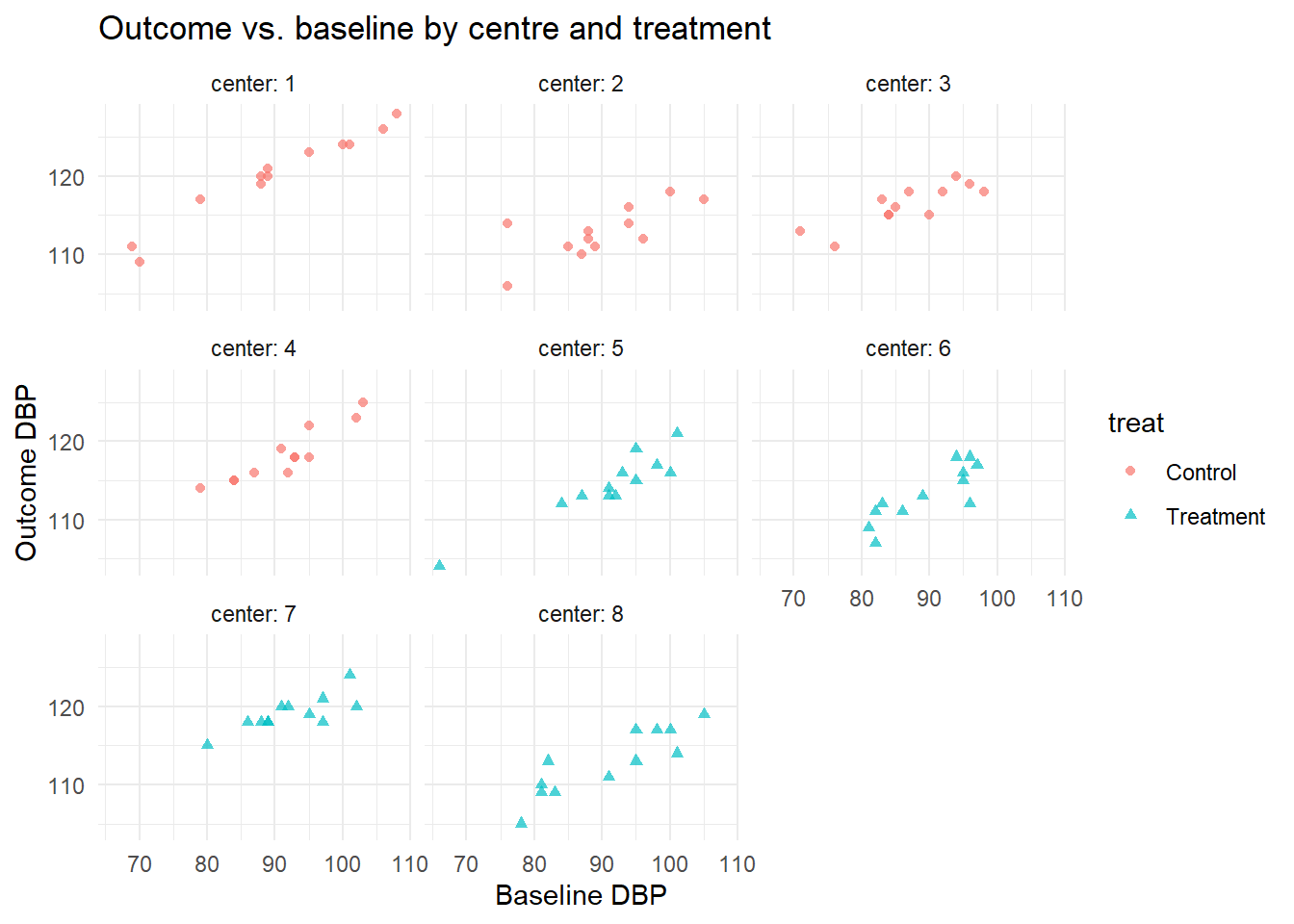
The dataset dat (simulated, 96 observations, 8 centres, 12 per centre) contains:

Variable	Description
`dbp`	Diastolic blood pressure at end of trial (outcome)
`dbp1`	Baseline DBP (covariate)
`treat`	Treatment group (Control / Treatment)
`center`	Hospital identifier (1–8)

Research question: Does the treatment reduce DBP, adjusting for baseline DBP and accounting for centre clustering?

2.2 Step 1: Explore the data

str(dat)

'data.frame':   96 obs. of  5 variables:
 $ center: Factor w/ 8 levels "1","2","3","4",..: 1 1 1 1 1 1 1 1 1 1 ...
 $ b_i   : num  4.8 4.8 4.8 4.8 4.8 ...
 $ treat : Factor w/ 2 levels "Control","Treatment": 1 1 1 1 1 1 1 1 1 1 ...
 $ dbp1  : num  106 89 100 108 79 88 89 95 88 69 ...
 $ dbp   : num  126 121 124 128 117 120 120 123 119 111 ...

table(dat$center, dat$treat)

   
    Control Treatment
  1      12         0
  2      12         0
  3      12         0
  4      12         0
  5       0        12
  6       0        12
  7       0        12
  8       0        12

ggplot(dat, aes(x = dbp1, y = dbp, colour = treat, shape = treat)) +
  geom_point(alpha = 0.7) +
  facet_wrap(~ center, labeller = label_both) +
  labs(x = "Baseline DBP", y = "Outcome DBP",
       title = "Outcome vs. baseline by centre and treatment") +
  theme_minimal()

Notice how the cluster means shift across panels — this is the between-centre variation that $\sigma_b^2$ captures.

2.3 Step 2: Fit the random intercept model

library(lme4)
fit_ri <- lmer(dbp ~ treat + dbp1 + (1 | center), data = dat)
summary(fit_ri)

Linear mixed model fit by REML ['lmerMod']
Formula: dbp ~ treat + dbp1 + (1 | center)
   Data: dat

REML criterion at convergence: 410.7

Scaled residuals: 
    Min      1Q  Median      3Q     Max 
-2.0517 -0.5402 -0.0312  0.5520  3.4869 

Random effects:
 Groups   Name        Variance Std.Dev.
 center   (Intercept) 7.479    2.735   
 Residual             3.269    1.808   
Number of obs: 96, groups:  center, 8

Fixed effects:
               Estimate Std. Error t value
(Intercept)    82.67670    2.41427   34.24
treatTreatment -2.52023    1.96886   -1.28
dbp1            0.38193    0.02203   17.34

Correlation of Fixed Effects:
            (Intr) trtTrt
treatTrtmnt -0.395       
dbp1        -0.817 -0.016

How to read this output

Fixed effects — look for:

treatTreatment: the estimated treatment effect (negative = reduction in DBP). Is it clinically meaningful? Is the SE large relative to the estimate?
dbp1: association between baseline and outcome DBP within centres.

Random effects — look for:

center (Intercept) Variance: between-centre variability ($\hat{\sigma}_b^2$). Large value = centres differ substantially.
Residual Variance: within-centre variability ($\hat{\sigma}^2$).
ICC rule of thumb: ICC < 0.05 = weak clustering; 0.05–0.20 = moderate; > 0.20 = strong. Strong clustering means ignoring it would seriously inflate Type I error.

No p-values? lmer does not report p-values by default. Use lmerTest::lmer() for Satterthwaite-approximated p-values, or compute confidence intervals with confint(fit_ri).

2.4 Step 3: Reading the output — fixed effects

Fixed effects:
                  Estimate Std. Error t value
(Intercept)         ...
treatTreatment      ...
dbp1                ...

(Intercept): Expected DBP for a control patient with dbp1 = 0. Not directly interpretable (baseline 0 is outside the data range), but needed for prediction.
treatTreatment: The estimated treatment effect — the average reduction in DBP for treated vs. control patients at the same centre and same baseline. This is the primary quantity of interest.
dbp1: Each 1 mmHg higher baseline DBP is associated with this many mmHg higher outcome DBP, on average, within the same centre.

On average, the treatment reduces DBP by 3.18 mmHg, conditional on each patient's baseline DBP and which centre they were in

The treatment increases rather than reduces DBP by 3.18 mmHg on average, contradicting the direction of the negative sign

The negative sign shows that exactly 3.18 out of the 8 centres in the study recorded an average improvement from treatment

Since the t-statistic magnitude |−1.32| exceeds the 1.0 threshold, the treatment effect is statistically significant at α = 0.05

The estimate for treatTreatment is the conditional treatment effect: treated patients have, on average, 3.18 mmHg lower DBP than control patients at the same centre and same baseline. The negative sign means reduction. The t-value of −1.32 is well below 1.96, so this effect is not statistically significant at the 5% level — but significance is separate from interpretation.

Fixed vs. random effects interpretation

Fixed effects coefficients (e.g., treatTreatment) describe the population-average effect. They answer: “On average, across all centres, what is the effect of treatment?”

This is a conditional interpretation — conditional on the random effect being 0 (i.e., for a “typical” centre with $b_i = 0$).

2.5 Step 4: Reading the output — random effects

Random effects:
 Groups   Name        Variance Std.Dev.
 center   (Intercept) ...      ...
 Residual             ...      ...

center (Intercept) Variance: This is $\hat{\sigma}_b^2$. It quantifies how much centres differ in their average DBP, after accounting for treatment and baseline.
Residual Variance: This is $\hat{\sigma}^2$. Within-centre variation unexplained by the fixed effects.
ICC: Compute as $\hat{\sigma}_b^2 / (\hat{\sigma}_b^2 + \hat{\sigma}^2)$.

vc <- as.data.frame(VarCorr(fit_ri))
vc

       grp        var1 var2     vcov    sdcor
1   center (Intercept) <NA> 7.478508 2.734686
2 Residual        <NA> <NA> 3.268604 1.807928

sigma_b_sq <- vc$vcov[1]
sigma_sq   <- vc$vcov[2]
icc        <- sigma_b_sq / (sigma_b_sq + sigma_sq)
cat("Estimated ICC:", round(icc, 3), "\n")

Estimated ICC: 0.696

12.25 / 4.00 = 3.06

12.25 / (12.25 + 4.00) ≈ 0.75

4.00 / (12.25 + 4.00) ≈ 0.25

3.50 / (3.50 + 2.00) ≈ 0.64

ICC = σ²_b / (σ²_b + σ²) = 12.25 / (12.25 + 4.00) = 12.25 / 16.25 ≈ 0.75. Use the Variance column (not Std.Dev.) in the formula. ICC = 0.75 means 75% of total variance is between centres — very strong clustering. Two patients from the same centre correlate at 0.75 even before adjusting for anything.

2.6 Step 5: Compare to a model ignoring clustering

fit_ols <- lm(dbp ~ treat + dbp1, data = dat)

# Treatment SE: mixed model vs OLS
cat("Mixed model SE for treatment:",
    round(summary(fit_ri)$coefficients["treatTreatment", "Std. Error"], 4), "\n")

Mixed model SE for treatment: 1.9689

cat("OLS SE for treatment:        ",
    round(summary(fit_ols)$coefficients["treatTreatment", "Std. Error"], 4), "\n")

OLS SE for treatment:         0.6161

What you should observe

The OLS standard error for treatment is smaller than the mixed model SE — this is the underestimation of uncertainty caused by ignoring clustering. Treatment is assigned at the centre level (4 control centres, 4 treatment centres), so the real comparison involves only 8 cluster means. OLS treats 96 patients as 96 independent units and reports false precision. The mixed model correctly identifies that the effective sample size for the treatment comparison is the number of clusters, not the number of patients.

For the parameters in this simulation ($n=12$, ICC $\approx 0.75$): DEFF $= 1 + 11 \times 0.75 = 9.25$, so OLS SE is roughly $\sqrt{9.25} \approx 3 \times$ too small.

3 Guided Practice

Goal: Fit a random intercept model on a new dataset and extract the key quantities.

The dataset sim2 below has a different ICC. Fit the model, extract the ICC, and compare the treatment SE between the mixed model and OLS.

R is loading in the background — the exercises below will be interactive once the status bar disappears. You can read the concept sections above immediately.

Hints

Task 1: The random effect specification for a random intercept for center is (1 | center)
Task 2: vc2$vcov[1] is the random intercept variance; vc2$vcov[2] is the residual variance
Task 3: Note that sim2 assigns treatment within clusters — each centre has both treated and control patients (rep(c(0,1), 100) alternates within each centre). This is the opposite design from the worked example. With within-cluster treatment, OLS absorbs the between-cluster noise into the residuals, inflating its SE estimate. You may find OLS SE larger than the mixed model SE — this is expected and not a contradiction. The mixed model is more efficient in both designs; only the direction of OLS’s error changes.

4 Retrieval Challenge

Solve these without hints. Each block is independent.

Challenge 1: The output below is from a random intercept model. Compute the ICC manually and interpret it in one sentence.

Challenge 2: A researcher fits lmer(y ~ x + (1|group), data = d) and gets: - Fixed effect for x: estimate = 2.1, SE = 0.8 - After refitting with lm(y ~ x, data = d): SE for x = 0.3

What does this tell you about the data structure? What is the likely direction of the ICC?

Challenge 3: True or false — and explain why:

“If the random intercept variance $\sigma_b^2 = 0$, the mixed model is equivalent to ordinary linear regression.”

Model answers

Challenge 1:

icc <- 12.4 / (12.4 + 5.8)   # = 0.681

ICC = 0.68: 68% of total variance is attributable to between-group differences. Two random observations from the same group have a correlation of 0.68 — very strong clustering.

Challenge 2: The large discrepancy (SE 0.8 vs 0.3) indicates strong positive clustering. When clustering is positive, OLS drastically underestimates uncertainty for predictors that vary between groups. The ICC is likely high (≥ 0.3).

Challenge 3: True — but with a caveat. When $\sigma_b^2 = 0$, all random effects are zero and the model collapses to OLS. However, lme4 will not exactly reproduce lm output because REML estimation of the residual variance differs slightly from OLS. The key point is that the random intercept adds no information when there is no between-cluster variation.

5 Why-Questions (Elaborative Interrogation)

These questions target common misconceptions. Think carefully before revealing the answer.

Q1: “I have 8 centres. Why not just add center as a fixed effect dummy variable instead of a random effect?”

Answer:

Adding centre as a fixed effect estimates 7 dummy coefficients (one per centre minus reference). This is called the “no pooling” or “fixed effects” estimator. It has two problems:

Degrees of freedom: You spend 7 df estimating centre effects that you don’t care about (they are nuisance parameters). With small clusters, this substantially reduces power.
No borrowing of information: Each centre is estimated in isolation. A centre with only 3 patients gets an imprecise estimate with no shrinkage. Random effects partially pool information across centres — centres with fewer observations are shrunk more towards the grand mean. This is the BLUP (Best Linear Unbiased Predictor) property.
No generalisation: Fixed centre effects describe these 8 centres only. Random effects assume centres are a sample from a population of centres — allowing inference to other centres not in the study.

When to use fixed instead of random? If you have few groups (< 5), or if you are explicitly interested in the group effects themselves, or if the independence assumption $b_i \perp \mathbf{x}_{ij}$ is violated (e.g., in economics panel data with time-varying treatments — use the Hausman test).

Q2: “The p-value for the treatment effect is large in the mixed model but small in the OLS. Which do I trust?”

Answer:

Trust the mixed model p-value.

The OLS p-value is anti-conservative: it uses underestimated SEs, so even random noise can appear significant. The smaller OLS p-value is a false positive inflated by the unaccounted clustering.

This is not a property of the specific dataset — it holds in expectation. Under $H_0$ (no treatment effect), a correctly specified mixed model maintains Type I error at $\alpha = 0.05$; OLS with clustered data can have Type I error of 0.3–0.5 depending on ICC.

This is why ignoring clustering is not just a theoretical concern — it is a reproducibility problem.

Q3: “The random intercepts are not a parameter I estimate — so why do they appear in the model?”

Answer:

The random effects $b_i$ are not fixed parameters — they are latent variables (unobserved). The model parameters are $\boldsymbol{\beta}$, $\sigma_b^2$, and $\sigma^2$. These are estimated by REML or ML.

The individual $b_i$ values are predicted (not estimated) using BLUPs:

\[\hat{b}_i = \hat{\sigma}_b^2 \mathbf{Z}_i^\top \hat{\mathbf{V}}_i^{-1} (\mathbf{y}_i - \mathbf{X}_i \hat{\boldsymbol{\beta}})\]

BLUPs shrink towards zero — the smaller the cluster and the smaller $\sigma_b^2$ relative to $\sigma^2$, the more shrinkage. This is a form of empirical Bayes estimation.

Practical consequence: ranef(fit_ri) gives predicted BLUPs, not estimated parameters. The uncertainty in BLUPs is larger than the uncertainty in $\hat{\boldsymbol{\beta}}$ and should not be ignored.

6 Spaced Review

These short questions revisit earlier material from the course to strengthen long-term retention. They appear at the end of each section and mix topics.

Review answers

Gauss-Markov conditions: 1. Linearity: $E[\mathbf{y}] = \mathbf{X}\boldsymbol{\beta}$ 2. Full rank: $\mathbf{X}$ has rank $p$ 3. Strict exogeneity: $E[\varepsilon | \mathbf{X}] = 0$ 4. Homoscedasticity: $\text{Var}(\varepsilon_i) = \sigma^2$ 5. No autocorrelation: $\text{Cov}(\varepsilon_i, \varepsilon_j) = 0$ for $i \neq j$

Clustering violates condition 5: observations within the same cluster have $\text{Cov}(Y_{ij}, Y_{ij'}) = \sigma_b^2 > 0$.

ICC formula: \[\text{ICC} = \frac{\sigma_b^2}{\sigma_b^2 + \sigma^2} = \frac{9}{9+6} = \frac{9}{15} = 0.6\]

Section summary

Concept	Formula / key fact
Random intercept model	$Y_{ij} = \mathbf{x}_{ij}^\top\boldsymbol{\beta} + b_i + \varepsilon_{ij}$
Random effect distribution	$b_i \sim \mathcal{N}(0, \sigma_b^2)$
ICC	$\rho = \sigma_b^2 / (\sigma_b^2 + \sigma^2)$
Effect of ignoring clustering	SE underestimated → inflated Type I error
Fixed vs. random effects	Fixed: estimates group effects; Random: borrows strength, generalises
Estimation	REML for variance components; ML for model comparison
`lme4` syntax	`lmer(y ~ x + (1 \| group), data = d)`