CS1.4 — Random Slopes

1 Before You Start

Recall: the random intercept model (CS1.2)

The random intercept model adds a group-specific shift to the regression:

\[Y_{ij} = (\beta_0 + b_i) + \beta_1 x_{ij} + \varepsilon_{ij}, \quad b_i \sim \mathcal{N}(0, \sigma_b^2)\]

Every group shares the same slope $\beta_1$ — only the baseline shifts. This chapter relaxes that assumption by also letting the slope vary across groups.

Recall: REML vs ML for model comparison (CS1.3)

Use ML (REML=FALSE) when comparing models via LRT — whether you are comparing fixed effects structures or random effects structures. Use REML (REML=TRUE) for final estimation and reporting variance components.

The standard workflow: (1) use ML for the LRT, (2) refit the preferred model with REML.

Recall: reading VarCorr() output (CS1.2)

VarCorr(fit) prints the estimated variance components:

Element	What it is
`(Intercept)` Std.Dev.	$\hat{\sigma}_{b_0}$ — SD of the random intercepts across groups
A slope’s Std.Dev.	$\hat{\sigma}_{b_1}$ — SD of the random slopes across groups
`Corr`	$\hat{\rho}$ — correlation between each group’s intercept and slope
`Residual` Std.Dev.	$\hat{\sigma}$ — within-group residual SD

Use as.data.frame(VarCorr(fit)) for a tidy table. Check isSingular(fit) to detect if any variance component is estimated at its boundary (0 or ±1).

2 Concept: When Slopes Also Vary

2.1 Extending the random intercept model

The random intercept model allows each group to have a different baseline level but assumes the effect of all predictors is identical across groups. This may be unrealistic. In our trial:

The treatment effect might be larger in some centres than others (centre-level moderators)
The relationship between baseline DBP and outcome might differ by centre

The random slope model extends the specification to let one or more slopes also vary:

\[Y_{ij} = (\beta_0 + b_{0i}) + (\beta_1 + b_{1i}) x_{ij} + \beta_2 z_{ij} + \varepsilon_{ij}\]

where: \[\begin{pmatrix} b_{0i} \\ b_{1i} \end{pmatrix} \sim \mathcal{N}\left(\begin{pmatrix}0\\0\end{pmatrix},\ \begin{pmatrix}\sigma_{b_0}^2 & \rho\sigma_{b_0}\sigma_{b_1} \\ \rho\sigma_{b_0}\sigma_{b_1} & \sigma_{b_1}^2\end{pmatrix}\right)\]

The correlation $\rho$ between random intercept and slope is estimated from the data. It captures, e.g., whether centres with higher baseline DBP also have steeper treatment responses.

2.2 Variance-covariance structure

The full random effects covariance matrix $\mathbf{G}$ is a $2 \times 2$ matrix per group. Across $m$ groups:

\[\mathbf{G}_{block} = \begin{pmatrix}\sigma_{b_0}^2 & \rho\sigma_{b_0}\sigma_{b_1} \\ \rho\sigma_{b_0}\sigma_{b_1} & \sigma_{b_1}^2\end{pmatrix}\]

This introduces 3 new parameters ($\sigma_{b_0}^2$, $\sigma_{b_1}^2$, $\rho$) compared to the random intercept model. Identifiability requires sufficient groups — estimating $\rho$ reliably needs $m \geq 10$–20 groups.

The model must be refit using maximum likelihood (ML) rather than REML for all estimation stages and not just when performing model comparisons

All fixed-effect coefficient estimates become biased and inconsistent whenever a random slope is added but there is insufficient cluster-level data

Two extra parameters (slope variance and intercept–slope covariance) must be estimated, so more data per cluster is needed to identify them reliably

The standard ICC formula based on intercept variance σ²_b and residual variance σ² can no longer be computed once random slopes are included

A random slope adds two parameters: the variance of the slopes (σ²_slope) and the covariance between intercepts and slopes. With few observations per cluster, these are poorly identified — leading to singular fits or estimates at boundary values (variance = 0, correlation = ±1).

2.3 `lme4` syntax

Model	Syntax
Random intercept only	`(1 \| group)`
Random intercept + slope, with correlation	`(1 + x \| group)`
Random intercept + slope, no correlation	`(1 \| group) + (0 + x \| group)`
Random slope only (no intercept)	`(0 + x \| group)`

Interpretational difference

Random intercept: “each group has its own baseline, but the slope of $x$ is the same everywhere”
Random slope: “each group has its own relationship between $x$ and $y$”

The fixed effect $\beta_1$ is now the average slope across groups. The random slope $b_{1i}$ describes how group $i$ deviates from this average.

Always — random slopes are strictly more flexible and cannot hurt

Only when the fixed effect of x is statistically significant

When the effect of x plausibly varies across clusters in the population of interest

Only when the ICC exceeds 0.3

A random slope is a substantive claim: the relationship between x and y is not the same in every cluster. This should be motivated by domain knowledge or the research question. Adding random slopes without sufficient data per cluster leads to singular fits and unreliable estimates.

2.4 Visualising random slopes

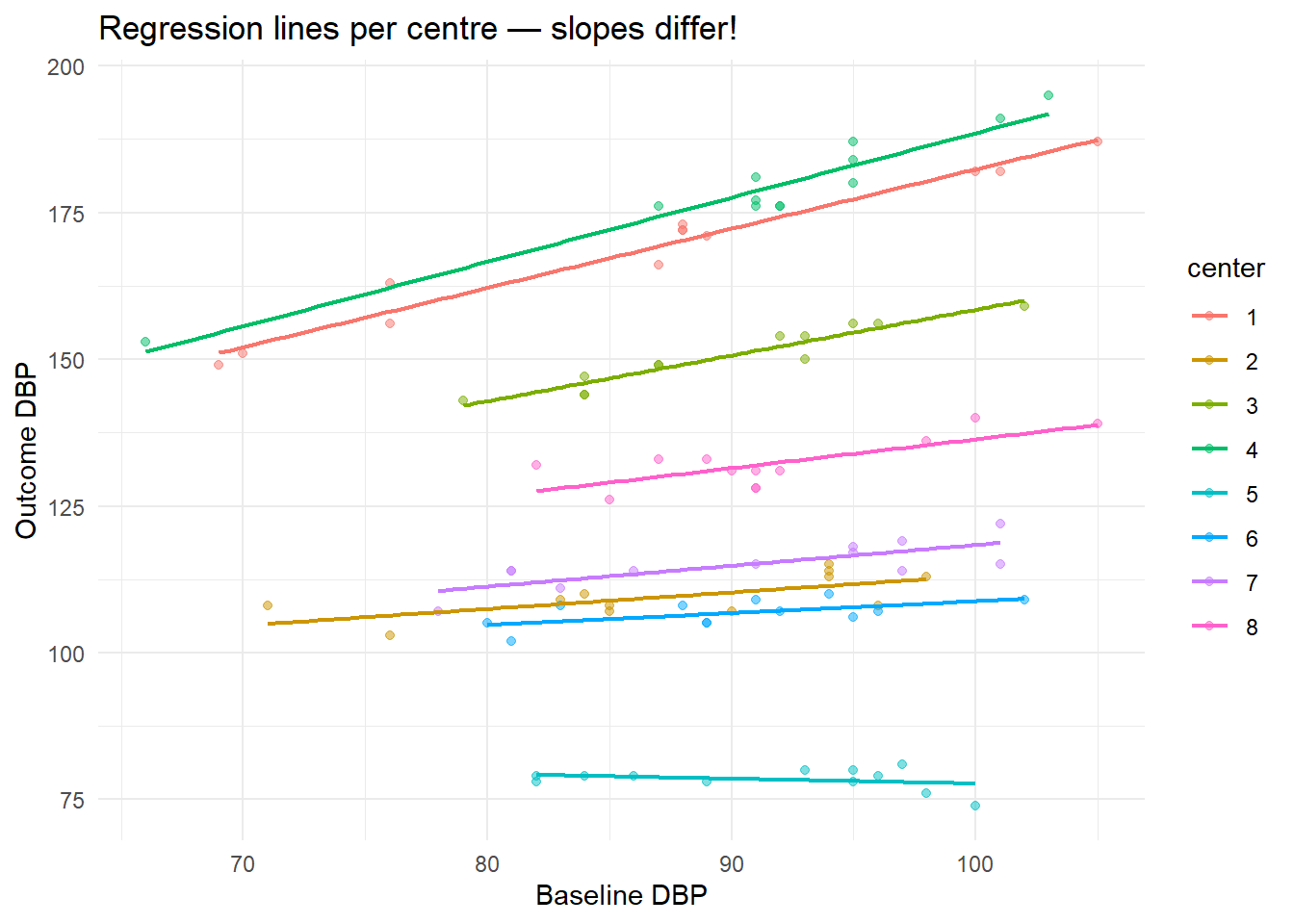
ggplot(dat, aes(x=dbp1, y=dbp, colour=center)) +
  geom_point(alpha=0.5, size=1.5) +
  geom_smooth(method="lm", se=FALSE, linewidth=0.8) +
  labs(title="Regression lines per centre — slopes differ!",
       x="Baseline DBP", y="Outcome DBP") +
  theme_minimal()

`geom_smooth()` using formula = 'y ~ x'

What to notice

The per-centre regression lines have different slopes — evidence that a random slope for dbp1 may be warranted. If all lines were parallel, a random intercept would suffice.

Clusters with higher baseline outcomes tend to show weaker (or reversed) effects of x

The model is misspecified and the correlation should be constrained to zero

The random intercept and slope cannot both be identified and one should be dropped

The fixed effect of x must be negative

A negative intercept–slope correlation (e.g., a ceiling effect) is substantively meaningful: groups that start high have less room to improve. This is a real, interpretable feature of the data — not a model failure. It should be reported and explained in context.

3 Worked Example

# Random intercept only
fit_ri <- lmer(dbp ~ treat + dbp1 + (1|center), data=dat, REML=TRUE)

# Random intercept + slope for dbp1
fit_rs <- lmer(dbp ~ treat + dbp1 + (1 + dbp1|center), data=dat, REML=TRUE)

boundary (singular) fit: see help('isSingular')

summary(fit_rs)

Linear mixed model fit by REML ['lmerMod']
Formula: dbp ~ treat + dbp1 + (1 + dbp1 | center)
   Data: dat

REML criterion at convergence: 458.3

Scaled residuals: 
    Min      1Q  Median      3Q     Max 
-2.1138 -0.7530 -0.0571  0.5880  3.3600 

Random effects:
 Groups   Name        Variance Std.Dev. Corr  
 center   (Intercept) 4.7775   2.1858         
          dbp1        0.1654   0.4067   -1.00 
 Residual             3.6342   1.9064         
Number of obs: 96, groups:  center, 8

Fixed effects:
               Estimate Std. Error t value
(Intercept)     84.0627     2.3622  35.587
treatTreatment  -2.6749     0.3898  -6.861
dbp1             0.5287     0.1459   3.623

Correlation of Fixed Effects:
            (Intr) trtTrt
treatTrtmnt -0.028       
dbp1        -0.482 -0.010
optimizer (nloptwrap) convergence code: 0 (OK)
boundary (singular) fit: see help('isSingular')

# Extract variance-covariance of random effects
VarCorr(fit_rs)

 Groups   Name        Std.Dev. Corr   
 center   (Intercept) 2.1858          
          dbp1        0.4067   -1.000 
 Residual             1.9064

Reading VarCorr() output for a random slope model

Element in output	What it means
`(Intercept)` Std.Dev.	$\hat{\sigma}_{b_0}$ — how much groups differ in their baseline level
`dbp1` Std.Dev.	$\hat{\sigma}_{b_1}$ — how much groups differ in their dbp1 slope; near 0 means slopes are similar everywhere
`Corr`	$\hat{\rho}$ — negative = high-baseline centres have flatter slopes; positive = high-baseline centres have steeper slopes
`Residual` Std.Dev.	$\hat{\sigma}$ — within-group noise after accounting for both fixed effects and random effects

If isSingular(fit_rs) returns TRUE, one variance component hit its boundary — the random slope adds no information and the simpler random-intercept model is likely sufficient.

Groups   Name        Std.Dev.  Corr
center   (Intercept)  3.49
         dbp1          0.28    -0.71
Residual               2.02

The model has a convergence problem — the correlation should be constrained to zero

The random intercept and slope explain the same variance and one is redundant

Centres with higher baseline DBP tend to have a weaker (flatter) relationship between dbp1 and outcome

The fixed effect of dbp1 is negative

Corr = −0.71 is the estimated correlation between each centre's random intercept and random slope. Negative means centres that start high (positive b₀) tend to have smaller slopes (negative b₁) — consistent with a ceiling effect. This is a substantive, interpretable finding, not a model error.

The slope is essentially the same in every centre — Std.Dev. = 0.28 is negligibly small and the random slope adds nothing useful to the model

Most centres (within ±2 SD) have slopes roughly between 0.40 − 2×0.28 = −0.16 and 0.40 + 2×0.28 = 0.96 — practically meaningful variation

The slope is negative in some centres because any positive Std.Dev. implies some groups must have slopes below zero if the distribution is symmetric

A Std.Dev. of 0.28 indicates high estimation uncertainty in the slope and the random slope component should be removed from the final model

The fixed effect β̂ = 0.40 is the average slope across all centres. The random slope Std.Dev. = 0.28 describes how much centres deviate from that average. About 95% of centres fall within β̂ ± 2·SD = −0.16 to 0.96. Since this range is wide — some centres show almost no association, others a strong one — there is meaningful variation worth modelling.

# Compare via LRT (use ML for fixed effects, same here)
fit_ri_ml <- lmer(dbp ~ treat + dbp1 + (1|center),         data=dat, REML=FALSE)
fit_rs_ml <- lmer(dbp ~ treat + dbp1 + (1+dbp1|center),    data=dat, REML=FALSE)
anova(fit_ri_ml, fit_rs_ml)

Data: dat
Models:
fit_ri_ml: dbp ~ treat + dbp1 + (1 | center)
fit_rs_ml: dbp ~ treat + dbp1 + (1 + dbp1 | center)
          npar    AIC    BIC  logLik -2*log(L)  Chisq Df Pr(>Chisq)    
fit_ri_ml    5 588.73 601.55 -289.36    578.73                         
fit_rs_ml    7 473.44 491.39 -229.72    459.44 119.29  2  < 2.2e-16 ***
---
Signif. codes:  0 '***' 0.001 '**' 0.01 '*' 0.05 '.' 0.1 ' ' 1

Reading the LRT output for a random slope

The output compares the two models row by row. Key columns:

Column	Meaning
`Df`	Number of estimated parameters — the random slope model has 2 more: $\hat{\sigma}_{b_1}^2$ and $\hat{\rho}$
`AIC` / `BIC`	Lower = better; both penalise the extra parameters — if they point in opposite directions, prefer the simpler model
`Chisq`	LRT statistic = $2(\ell_{\text{RS}} - \ell_{\text{RI}})$
`Pr(>Chisq)`	p-value — but conservative: $H_0: \sigma_{b_1}^2 = 0$ sits on the boundary of the parameter space, so the true p-value is roughly half what is printed

          Df   AIC    BIC   logLik  Chisq  Chi Df  Pr(>Chisq)
fit_ri_ml  5  498.3  514.1  -244.2
fit_rs_ml  7  497.8  516.8  -241.9   4.56      2       0.102

The random slope is not warranted — p = 0.102 already exceeds 0.05 and BIC also disfavours RS, making the RI model the clearly preferred choice

The random slope is clearly supported — any AIC improvement is sufficient to justify added parameters and the p-value is close to significance

After boundary correction p ≈ 0.05 and criteria disagree — retain the random slope only if theory clearly predicts between-centre slope variation

The LRT is invalid here — testing a random slope variance requires df = 1, not df = 2, so the Chisq and p-value in the output cannot be interpreted

Testing H₀: σ²_{b₁} = 0 is a boundary test — the corrected p-value is approximately 0.102 / 2 = 0.051. AIC (−0.5 difference) barely favours RS; BIC (−2.7) favours the simpler RI model. With such marginal evidence, the decision should lean on domain knowledge: if there is a prior reason to expect centres to differ in their dbp1 slope, keep the random slope. If not, the simpler RI model is defensible.

Interpreting the test

The LRT tests $H_0: \sigma_{b_1}^2 = 0$ (and $\rho = 0$). This is a boundary test (df = 2, mixture distribution). A non-significant result means the data are consistent with a random intercept model. However, if theory suggests slopes should vary, retain the random slope even if non-significant — it protects against anti-conservative inference.

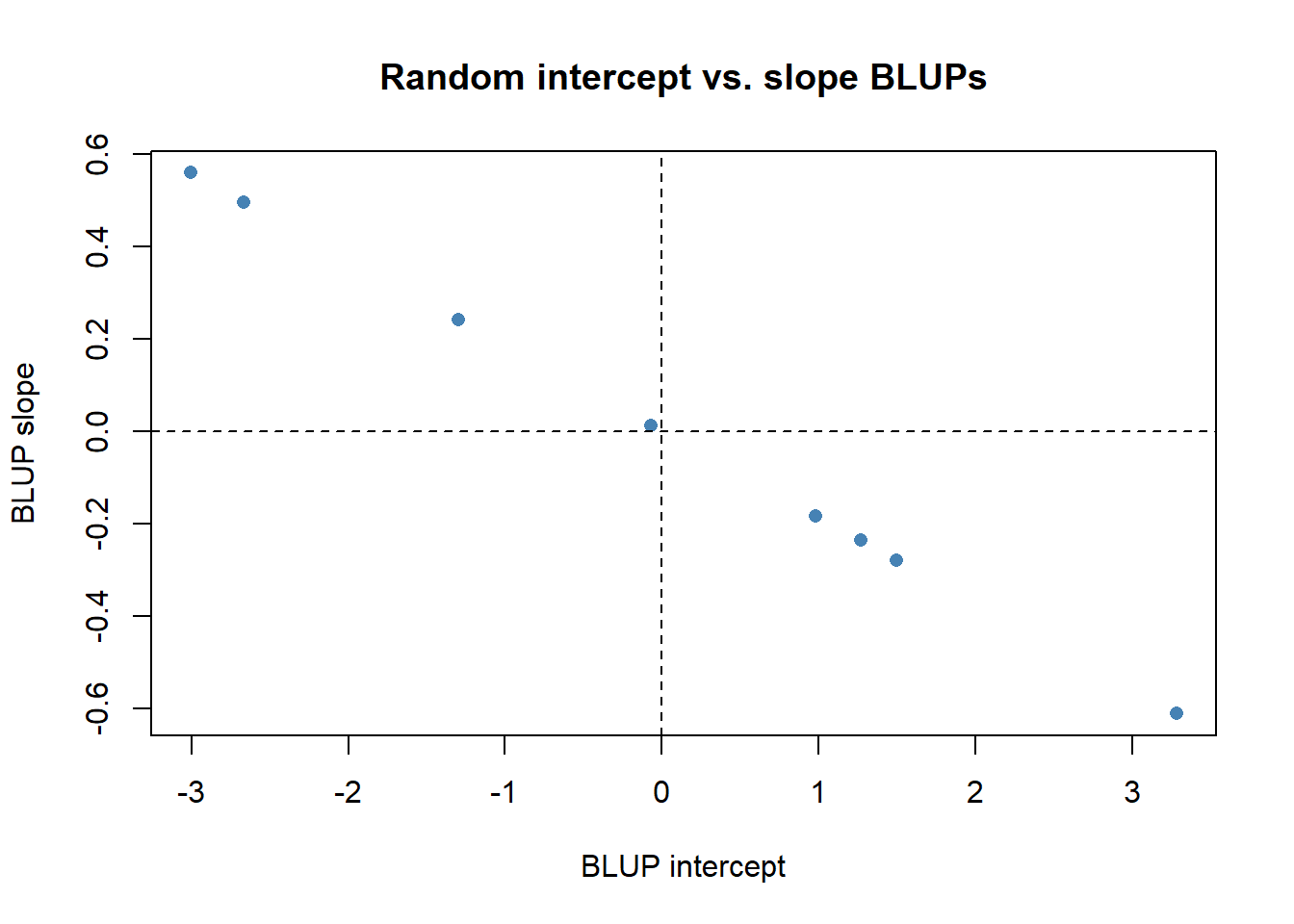
# Extract predicted random effects (BLUPs)
re <- ranef(fit_rs)$center
colnames(re) <- c("BLUP_intercept","BLUP_slope")
round(re, 3)

  BLUP_intercept BLUP_slope
1         -2.666      0.496
2          1.271     -0.237
3         -1.295      0.241
4         -3.006      0.559
5          3.285     -0.611
6          1.497     -0.279
7          0.983     -0.183
8         -0.070      0.013

# Plot: are intercept and slope BLUPs correlated?
plot(re[,1], re[,2],
     xlab="BLUP intercept", ylab="BLUP slope",
     main="Random intercept vs. slope BLUPs",
     pch=16, col="steelblue")
abline(h=0, v=0, lty=2)

4 Guided Practice

R is loading in the background — the exercises below will be interactive once the status bar disappears. You can read the concept sections above immediately.

Hints

Random slope for time: (1 + time | school)
Use REML=FALSE for comparison, then refit with REML=TRUE
ranef(fit)$school gives BLUPs; cor(ranef(fit)$school) gives correlations

5 Retrieval Challenge

Model answers

Q1: Corr = −0.85 means groups with higher intercepts tend to have more negative (smaller) slopes — e.g., schools starting at higher levels improve more slowly.

Q2: When you have few groups (< 10), estimating $\rho$ is unreliable. Use (1|group) + (0+x|group) to constrain correlation to 0 and reduce the number of estimated parameters.

Q3: With mean slope 1.5 and SD 0.2, most groups (±2 SD) have slopes between 1.1 and 1.9. Over x = 0–10, this translates to predicted Y differences of 11 to 19 — practically meaningful variation.

6 Why-Questions

Q: “My model with random slopes doesn’t converge. What should I do?”

Convergence failures in lme4 are common with complex random effects and small data. In order:

Scale your predictors — scale(x) before fitting. Convergence problems often arise from variables on very different scales.
Simplify the random structure — remove the correlation parameter first ((1|g) + (0+x|g)), then consider dropping the random slope altogether.
Change the optimizer — try control = lmerControl(optimizer = "bobyqa").
Check if the model is overparameterised — if $m < 10$ groups, random slopes may not be identifiable.

A convergence warning does not always mean the estimates are wrong — check whether the gradient is small and the Hessian is positive definite (isSingular(fit)).

Q: “isSingular() returned TRUE. Should I be worried?”

A singular fit means at least one variance component is estimated at 0 (or a correlation at ±1). This indicates the model is more complex than the data can support — the random effect you added contributes nothing. Options:

Drop the random slope (or the random intercept if it’s the singular component)
Use a Bayesian model with a regularising prior on variance components
Accept the singular fit if the fixed effects are stable — singular random effects still protect fixed-effect SEs from being anti-conservative

7 Spaced Review

Review answer

Use REML=FALSE — comparing random effects structures requires ML (or a specialised REML-based test). lme4’s anova() will warn and refit with ML automatically if you pass REML fits, but it’s cleaner to specify it explicitly.