Many outcomes in medicine and social science are not just categorical — they are ranked. Pain is rated from none to severe. Recovery is classified as none, partial, or complete. Satisfaction is recorded on a scale from strongly disagree to strongly agree. These are ordinal outcomes: the categories have a meaningful order, but the distances between them are not necessarily equal.
The multinomial logistic regression model covered in CS2 treats all categories as unordered. Applied to an ordinal outcome, it works — but it throws away the information contained in the ranking. A model that respects the ordering can use that information to estimate a single effect for each predictor rather than one per category comparison, leading to more efficient and interpretable results.
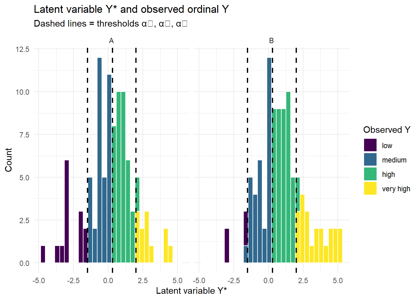
A useful way to think about ordinal outcomes is through a latent variable framework: imagine there is an underlying continuous measure (e.g., true health status) that gets cut into ordered categories by thresholds. The observed ordinal outcome is a coarsened version of that latent variable. This framing motivates the cumulative logit (proportional odds) model introduced in CS3.2.
On this page you will see why ordinal structure matters, how the latent variable idea works, and what assumptions underlie ordinal regression.
NoteAbbreviations used on this page
Abbreviation
Full term
PO
Proportional odds
CLM
Cumulative link model
OR
Odds ratio
LRT
Likelihood ratio test
1 Concept: When Categories Have an Order
1.1 Ordered vs unordered categories
The multinomial model (CS2) treats all categories as unordered — it makes no use of any ranking among them. When categories have a natural order, this discards information.
Treating these as nominal (using multinomial regression) is valid but inefficient: the model estimates \(K-1\) separate slopes for each predictor, when a single slope might suffice.
Ordinal regression is faster to compute and always gives smaller p-values for the predictor effects of interest
Multinomial regression cannot handle outcomes with more than 4 categories, requiring a different modelling approach
Ordinal regression exploits the ranking to estimate a single slope, gaining efficiency over K−1 separate slopes
Ordinal regression does not require selecting a reference category the way baseline-category logit models do
Multinomial regression estimates K−1 separate coefficient vectors — one per non-reference category. If the outcome is ordered, this discards information about the ranking and wastes degrees of freedom. The proportional odds model estimates a single β shared across all cumulative equations, which is more efficient when the ordering is informative.
1.2 The latent variable framework
A key insight for ordinal models: imagine that the ordered response \(Y\) arises from an unobserved continuous latent variable\(Y^*\):
The choice of \(F\) gives different models: - \(F\) = logistic CDF → proportional odds (cumulative logit) model - \(F\) = standard normal CDF → ordered probit model
ImportantWhat the latent variable represents
In pain research, \(Y^*\) might represent true pain intensity, which is continuous but we can only observe it in categories. In quality-of-life research, it is a latent construct. The thresholds represent the “cut-off” levels at which perception crosses into the next response category.
The regression coefficients for each predictor in each category
The cut-off values on the latent scale at which the observed category changes
The predicted probabilities for each category at the mean predictor value
The variance components of the latent variable
The latent variable Y* is continuous. We observe Y = k when α_{k-1} < Y* ≤ α_k. The thresholds are the boundaries on the latent scale separating adjacent categories. More widely spaced thresholds mean the categories are more distinct; narrowly spaced thresholds indicate categories are hard to distinguish.
# Effect of x on latent variable shifts the distribution → different category proportionsx_low <- dat[dat$x <-1,]x_high <- dat[dat$x >1,]cat("Category proportions for x < -1:\n")
Category proportions for x < -1:
round(prop.table(table(x_low$y_ord)), 3)
      low    medium      high very high
    0.407     0.519     0.074     0.000
cat("\nCategory proportions for x > 1:\n")
Category proportions for x > 1:
round(prop.table(table(x_high$y_ord)), 3)
      low    medium      high very high
    0.000     0.000     0.258     0.742
TipWhat to notice
A positive coefficient shifts the latent distribution to the right, increasing the probability of higher categories. The same shift applies everywhere — this is the proportional odds assumption (explored in CS3.3).
The proportional odds model, which uses the logistic CDF instead of the normal CDF as its error distribution
The multinomial logistic model, which does not use a latent variable framework and treats categories as unordered
The ordered probit model — because the probit link uses the normal CDF as its inverse link function
The cumulative complementary log-log model, which uses the Gumbel extreme value distribution as its error CDF
The choice of F determines the link function. F = logistic CDF → proportional odds (logit link). F = normal CDF → ordered probit (probit link). F = Gumbel (extreme value) CDF → complementary log-log link. The proportional odds model is most commonly used because the OR interpretation is natural and the logit is symmetric.
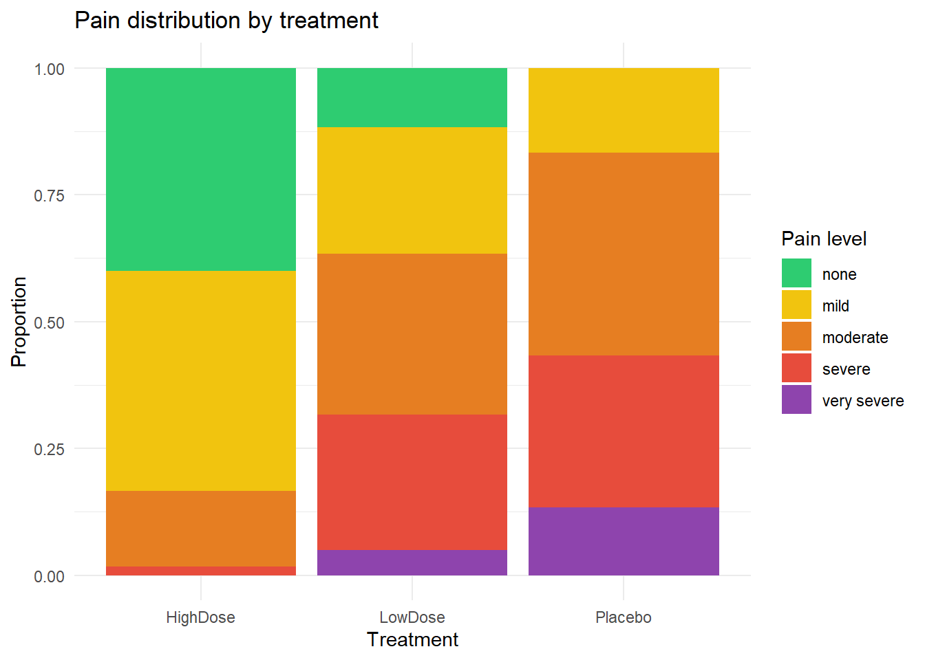
           none mild moderate severe very severe
  HighDose   24   26        9      1           0
  LowDose     7   15       19     16           3
  Placebo     0   10       24     18           8
ggplot(pain_dat, aes(x=treatment, fill=pain)) +geom_bar(position="fill") +scale_fill_manual(values=c("#2ecc71","#f1c40f","#e67e22","#e74c3c","#8e44ad")) +labs(title="Pain distribution by treatment",x="Treatment", y="Proportion", fill="Pain level") +theme_minimal()
The stacked bar chart shows the marginal distribution of pain by treatment group. The ordinal model will quantify the shift formally, adjusting for age.
3 Guided Practice
R is loading in the background — the exercises below will be interactive once the status bar disappears. You can read the concept sections above immediately.
TipHints
cut(surv$wait, quantile(surv$wait, c(0,.25,.5,.75,1)), include.lowest=TRUE) for quartiles
Consider: is satisfaction truly ordered? Is the gap between 1 and 2 the same as between 4 and 5?
4 Retrieval Challenge
NoteModel answers
Q1:\(\alpha_k\) is the value of the latent variable \(Y^*\) at which the response transitions from category \(k\) to \(k+1\). If \(\alpha_2 = 1.5\), then \(Y^* \leq 1.5\) maps to categories 1 or 2, and \(Y^* > 1.5\) maps to categories 3 or higher.
Q2: Yes — ordinal models don’t require equal spacing of categories (that’s the interval scale assumption). You’re only assuming the ranking is meaningful. Skipping a label doesn’t violate the model; it just means the threshold between “mild” and “severe” may be wide.
Q3: A shift changes probabilities of all categories — higher categories increase, lower categories decrease. The ordinal structure ensures these changes are internally consistent (they sum to 0).
5 Why-Questions
CautionQ: “Why not just treat the ordinal outcome as continuous and use linear regression?”
Treating ordered categories as continuous (e.g., coding none=0, mild=1, moderate=2, severe=3) implies: 1. Equal spacing between categories — the difference between none and mild is the same as between moderate and severe 2. Normally distributed residuals — unlikely for a bounded 4-point scale 3. Predicted values can be negative or > 3 — nonsensical
In large, well-powered studies, linear regression on ordinal outcomes can still give approximately valid inference for the slope (it’s a pseudo-effect of sorts). But the predicted values and standard errors will be wrong, and the equal-spacing assumption is rarely defensible.
CautionQ: “What is the difference between the ordinal logistic model and the ordinal probit model?”
Both use the latent variable framework but differ in the assumed distribution of \(\varepsilon\): - Logistic (\(F\) = logistic CDF): heavier tails than normal; gives proportional odds model; ORs are directly interpretable - Probit (\(F\) = standard normal CDF): slightly lighter tails; common in econometrics; gives probit effects
In practice, for most datasets, the two give nearly identical predictions and inferences. Choose logistic if you want OR interpretation; probit if you want to model a normally distributed latent variable or connect to structural equation models.
6 Spaced Review
NoteFurther reading
Agresti, A. (2010). Analysis of Ordinal Categorical Data (2nd ed.). Wiley. — Chapter 3.