CS3.5 — Predictions & Model Extensions

0.1 What this page is about

Coefficients and odds ratios (ORs) describe relative effects, but clinical and practical decisions require absolute probabilities: given this patient’s profile, how likely are they to be in each category of the outcome?

In the proportional odds (PO) model, predictions work by first computing the linear predictor — the weighted sum of predictor values times their coefficients — and then using it to shift all cumulative probabilities simultaneously. Because the same linear predictor appears in every cumulative equation, changing a predictor value shifts the entire probability distribution up or down the ordinal scale in one movement. The result is a complete predicted probability for every outcome category.

A practical consequence: unlike linear regression, the absolute change in probability for a given predictor shift depends on where on the scale you currently are. A predictor that shifts the linear predictor by 1 unit has a larger effect on probability in the middle of the distribution than at the extremes.

On this page you will learn how to use predict() with type = "probs", how to visualise predicted distributions across covariate profiles, and how the PO model can be extended for more complex settings.

Abbreviations used on this page

Abbreviation	Full term
PO	Proportional odds
OR	Odds ratio
CI	Confidence interval

1 Concept: Prediction and Model Extensions

1.1 Predicted probabilities from polr

The predicted category probability for profile \(\mathbf{x}_0\) is:

\[\hat{P}(Y = k | \mathbf{x}_0) = \text{logistic}(\hat{\alpha}_k - \hat{\boldsymbol{\beta}}^\top \mathbf{x}_0) - \text{logistic}(\hat{\alpha}_{k-1} - \hat{\boldsymbol{\beta}}^\top \mathbf{x}_0)\]

The linear predictor \(\hat{\boldsymbol{\beta}}^\top \mathbf{x}_0\) is the same for all cut-points — it shifts all cumulative probabilities simultaneously.

It changes only the predicted probability of the most likely category, leaving all other category probabilities unchanged

It changes each category's probability by the same absolute amount, since the PO model assumes equal spacing across categories

It shifts the entire distribution by moving the linear predictor β'x — all cumulative probabilities change in the same direction

It only affects the probabilities of the extreme categories (lowest and highest), leaving intermediate categories unchanged

The linear predictor β'x appears in all cumulative probability equations simultaneously: P(Y ≤ k) = logistic(α_k − β'x). Increasing x by 1 shifts β'x by β, which decreases all P(Y ≤ k) by a linked amount. This shifts probability mass from lower to higher categories uniformly — a key feature (and constraint) of the PO model.

1.2 Uncertainty in predictions: delta method

For a scalar function \(g(\hat{\boldsymbol{\theta}})\) (e.g., a predicted probability), the delta method gives:

\[\widehat{\text{SE}}(g(\hat{\boldsymbol{\theta}})) \approx \sqrt{\left(\frac{\partial g}{\partial \boldsymbol{\theta}}\bigg|_{\hat{\boldsymbol{\theta}}}\right)^\top \widehat{\text{Var}}(\hat{\boldsymbol{\theta}}) \left(\frac{\partial g}{\partial \boldsymbol{\theta}}\bigg|_{\hat{\boldsymbol{\theta}}}\right)}\]

Applied to a cumulative probability \(F(\alpha_k - \hat{\boldsymbol{\beta}}^\top\mathbf{x}_0)\), the gradient involves the logistic density evaluated at the linear predictor.

The CI is too wide — predictions in ordinal models should be more precise than this range, suggesting a model misspecification

The predicted probability falls near the extreme boundaries of (0,1), where the delta method gives unreliable interval estimates

The delta method assumes β̂ is approximately normal — in small samples or near boundary probabilities this approximation may be poor

Confidence intervals for ordinal regression cannot be computed without bootstrapping because the normal approximation always fails

The delta method propagates parameter uncertainty through a linear approximation. It works well when β̂ is approximately normal (large samples) and predicted probabilities are not near 0 or 1. For small samples or extreme predicted probabilities, the bootstrap provides a more reliable alternative — at the cost of computation time.

1.3 Extensions of the cumulative link model

The basic PO model can be extended in several directions:

Extension	What it adds
Partial PO	Some predictors have category-specific slopes
Scale model	Residual variance depends on covariates (heteroscedastic latent variable)
Location-scale	Both location (\(\boldsymbol{\beta}\)) and scale (\(\boldsymbol{\gamma}\)) modelled
Random effects	Clustered ordinal data (mixed ordinal model)

Some thresholds to be equal, simplifying the model

Some predictors to have category-specific slopes while others remain proportional across cut-points

The model to be fitted without specifying the number of categories in advance

Cluster-specific thresholds for multilevel ordinal data

Partial PO (e.g., Peterson-Harrell model) allows a subset of predictors to violate PO by estimating separate slopes for each cut-point, while others are constrained to be proportional. This is a middle ground between full PO (one slope per predictor) and full multinomial (K−1 slopes per predictor). The ordinal::clm function's `nominal` argument implements this.

2 Worked Example

# Predicted probabilities for specific profiles
newdat <- data.frame(ses  = c(1,1,1,0,0,0),
                     life = c(0,4,9,0,4,9))
preds <- predict(fit, newdata=newdat, type="probs")
rownames(preds) <- paste0("ses=",newdat$ses,",life=",newdat$life)
round(preds, 3)

              well  mild moderate impaired
ses=1,life=0 0.539 0.273    0.126    0.061
ses=1,life=4 0.235 0.298    0.267    0.199
ses=1,life=9 0.055 0.122    0.253    0.570
ses=0,life=0 0.371 0.315    0.199    0.115
ses=0,life=4 0.134 0.231    0.304    0.331
ses=0,life=9 0.028 0.069    0.178    0.725

                  well   mild  moderate  impaired
ses=1, life=0    0.511  0.218     0.145     0.126
ses=1, life=4    0.305  0.237     0.229     0.229
ses=1, life=9    0.122  0.168     0.253     0.457
ses=0, life=0    0.261  0.236     0.254     0.249
ses=0, life=4    0.122  0.168     0.253     0.457
ses=0, life=9    0.037  0.079     0.200     0.684

well (highest baseline probability)

moderate (middle category)

impaired — P(impaired) = 0.684 is by far the highest probability for that profile

mild — the model always puts most mass on intermediate categories

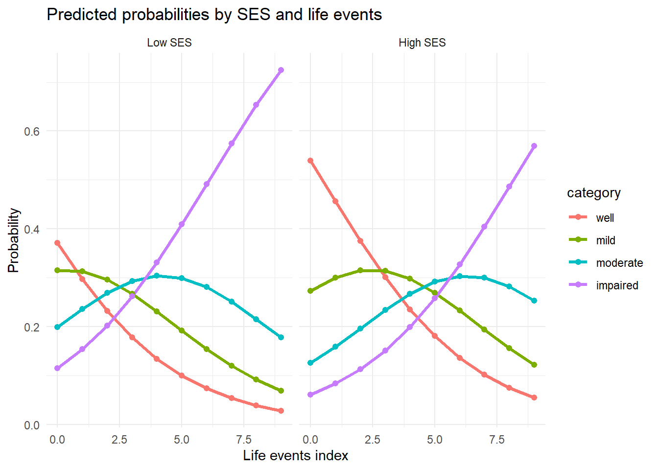
For ses=0 (low SES) and life=9 (many life events), P(impaired) = 0.684 — nearly 70% of the probability mass is in the worst category. Compare to ses=1, life=0: P(well) = 0.511, the most likely outcome is the best category. This contrast illustrates how both risk factors jointly push the distribution across all four categories. Notice that for every profile, the four probabilities sum to 1.

grid <- expand.grid(ses=0:1, life=0:9)
pred_g <- as.data.frame(predict(fit, newdata=grid, type="probs"))
pred_g$ses  <- factor(grid$ses, labels=c("Low SES","High SES"))
pred_g$life <- grid$life
pred_long <- pivot_longer(pred_g, -c(ses,life), names_to="category", values_to="prob")
pred_long$category <- factor(pred_long$category,
                              levels=c("well","mild","moderate","impaired"))

ggplot(pred_long, aes(x=life, y=prob, colour=category)) +
  geom_line(linewidth=1.2) + geom_point(size=1.8) +
  facet_wrap(~ses) +
  labs(title="Predicted probabilities by SES and life events",
       x="Life events index", y="Probability") +
  theme_minimal()

# Delta method CI for P(Y=well | ses=1, life=0)
x0     <- c(1, 0)      # ses=1, life=0
alphas <- fit$zeta      # thresholds
betas  <- coef(fit)    # coefficients

# Cumulative linear predictor for first threshold (well|mild)
lp    <- alphas[1] - sum(betas * x0)
p_cum <- plogis(lp)
cat("P(Y<=well | ses=1, life=0):", round(p_cum, 4), "\n")

P(Y<=well | ses=1, life=0): 0.5395

cat("= P(Y=well | ses=1, life=0):", round(p_cum, 4), "(since P(Y<well)=0)\n")

= P(Y=well | ses=1, life=0): 0.5395 (since P(Y<well)=0)

# Gradient: d(plogis(alpha1 - beta*x)) / d(beta, alpha1)
f_lp  <- dlogis(lp)   # logistic density at lp
# w.r.t. beta_ses:  -x0[1] * f_lp
# w.r.t. beta_life: -x0[2] * f_lp
# w.r.t. alpha1:    +1 * f_lp
grad <- c(f_lp, -x0 * f_lp)   # order: alpha1, beta_ses, beta_life

# Variance-covariance of (alpha1, beta_ses, beta_life)
vcov_mat <- vcov(fit)
# polr vcov: rows/cols ordered as coefficients then zeta
# Extract relevant submatrix
all_par <- c("ses","life","well|mild","mild|moderate","moderate|impaired")
idx <- c(3,1,2)   # alpha1=3rd in vcov, ses=1st, life=2nd
V_sub <- vcov_mat[idx, idx]

se_delta <- sqrt(t(grad) %*% V_sub %*% grad)
cat("\nSE (delta method):", round(se_delta, 4), "\n")


SE (delta method): 0.0701

cat("95% CI: [", round(p_cum - 1.96*se_delta, 4), ",",
               round(p_cum + 1.96*se_delta, 4), "]\n")

95% CI: [ 0.402 , 0.677 ]

3 Scale Extension

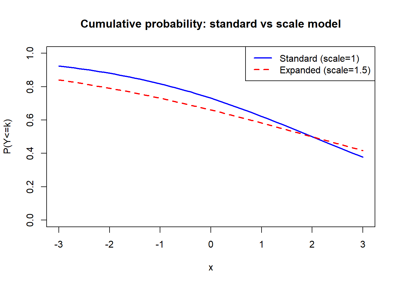
# The scale model allows the dispersion of the latent variable to depend on x:
# Y*_i ~ Location(mu_i, sigma_i) where log(sigma_i) = gamma * z_i
# This relaxes the assumption of constant variance in the latent variable.
#
# MASS::polr does not implement the scale model directly.
# The 'ordinal' package (if available) implements it via:
#   clm(y ~ x, scale = ~ z, data = dat)
#
# Conceptual example: what does a scale effect look like?
# If gamma > 0: observations with z=1 have MORE spread in the latent variable
# → thinner tails of each cumulative probability curve
# → probabilities are "less extreme" (closer to 1/K)

cat("Scale model concept:\n")

Scale model concept:

x_val <- seq(-3, 3, by=0.1)
# Standard (scale=1):
p_std   <- plogis(1.0 - 0.5*x_val)
# Expanded scale (scale=1.5):
p_scale <- plogis((1.0 - 0.5*x_val) / 1.5)

plot(x_val, p_std, type="l", col="blue", lwd=2,
     xlab="x", ylab="P(Y<=k)", main="Cumulative probability: standard vs scale model",
     ylim=c(0,1))
lines(x_val, p_scale, col="red", lwd=2, lty=2)
legend("topright", c("Standard (scale=1)","Expanded (scale=1.5)"),
       col=c("blue","red"), lty=c(1,2), lwd=2)

4 Guided Practice

R is loading in the background — the exercises below will be interactive once the status bar disappears. You can read the concept sections above immediately.

5 Retrieval Challenge

What to check

Cumulative probabilities must be increasing (always true if \(\alpha_1 < \alpha_2 < \alpha_3\))
Category probabilities must sum to 1
The absolute risk difference gives a more meaningful clinical summary than the OR alone

6 Why-Questions

Q: “I want to report a single number summarising the treatment effect. Should I report the OR or the predicted probability difference?”

Both are valid but answer different questions:

OR (from coefficient): multiplicative effect on the cumulative odds; constant under PO assumption; useful for comparing across studies with different baseline risks
Probability difference: absolute effect at a specific covariate profile; clinically interpretable; changes with covariate values

Best practice: report the OR (with CI) as the primary summary of the model, and supplement with predicted probabilities for clinically relevant profiles (e.g., “for a 60-year-old in treatment B vs A, P(excellent response) increases by X percentage points”).

Q: “How do mixed ordinal models work — when I have both clustering and an ordered outcome?”

The cumulative link mixed model (CLMM) extends the PO model with random effects:

\[\text{logit}\,P(Y_{ij} \leq k | \mathbf{x}_{ij}, b_i) = \alpha_k - \mathbf{x}_{ij}^\top\boldsymbol{\beta} - b_i, \quad b_i \sim \mathcal{N}(0,\sigma_b^2)\]

The random intercept \(b_i\) shifts the latent variable for cluster \(i\). In R: ordinal::clmm(y ~ x + (1|group), data=dat).

This combines CS1 (mixed model structure) with CS3 (ordinal outcome). The interpretation is the same as for CLMM: fixed effects are cluster-conditional (subject-specific), and the random effect captures unexplained between-cluster heterogeneity.

7 Full Course Review

# Choose the right model for each scenario — write your answers as comments

# Scenario 1: Patient response to treatment (none / partial / complete)
#             measured in a multi-centre trial (10 centres, 20 patients each)
# → Model: ?

# Scenario 2: Voter preference in an election (Labour / Conservative / Green / Other)
#             predicted by age, income, region
# → Model: ?

# Scenario 3: Self-rated health (poor / fair / good / very good / excellent)
#             in a cross-sectional survey with 5000 respondents
# → Model: ?

# Scenario 4: Same as Scenario 3, but you suspect the proportional odds
#             assumption is violated for the 'age' predictor
# → Model: ?

# Now verify your Scenario 3 answer with a simulation:
set.seed(100)
n_rev <- 500
d_rev <- data.frame(age=round(rnorm(500,45,15)), income=rnorm(500))
lat_rev <- 0.02*d_rev$age + 0.5*d_rev$income + rlogis(500)
d_rev$health <- ordered(cut(lat_rev, breaks=c(-Inf,-1,0,1,2,Inf),
                            labels=c("poor","fair","good","very good","excellent")),
                        levels=c("poor","fair","good","very good","excellent"))
fit_rev <- polr(health ~ age + income, data=d_rev, Hess=TRUE)
summary(fit_rev)

Call:
polr(formula = health ~ age + income, data = d_rev, Hess = TRUE)

Coefficients:
         Value Std. Error t value
age    0.01083   0.005267   2.057
income 0.39261   0.078345   5.011

Intercepts:
                    Value   Std. Error t value
poor|fair           -1.4764  0.2654    -5.5637
fair|good           -0.4667  0.2518    -1.8532
good|very good       0.5623  0.2521     2.2302
very good|excellent  1.7054  0.2623     6.5017

Residual Deviance: 1547.655 
AIC: 1559.655

exp(coef(fit_rev))   # ORs

     age   income 
1.010891 1.480836

Model answers

Scenario 1: Cumulative link mixed model (ordinal::clmm) — ordered outcome + clustering. Scenario 2: Multinomial logistic regression (nnet::multinom) — unordered, 4 categories. Scenario 3: Proportional odds model (polr or ordinal::clm) — large \(n\), ordered outcome. Scenario 4: Partial proportional odds, or full multinomial if the violation is severe. Test PO first via LRT; if violated for age only, allow age to have separate slopes per equation.