CS4.1 — Multiple Imputation & Rubin’s Rules

When data are missing, the simplest fix is to drop every incomplete row and analyse what remains. This complete case analysis (CC) is unbiased only when the data are missing completely at random — a strong assumption that is rarely met in practice. If older patients are more likely to miss a follow-up blood pressure measurement, dropping them removes a systematic slice of the data and biases every downstream estimate.

Multiple imputation (MI) addresses this by creating M complete versions of the dataset, each with the gaps filled by plausible values drawn from the observed patterns. The same analysis is run M times — once per completed dataset — producing M slightly different estimates. Rubin’s rules then pool these into a single result that accounts for both ordinary sampling uncertainty and the extra uncertainty that came from the missing data.

The pooling is the key challenge. Averaging the M estimates handles the point estimate, but the standard error needs more care: it must reflect two distinct sources of variation — uncertainty within each imputed dataset, and variation between the M datasets. Ignoring the second source gives confidence intervals (CIs) that are too narrow.

This page covers the complete pipeline: classifying your missing data mechanism (MCAR, MAR, or MNAR), running MI with the mice package, and working through Rubin’s pooling rules one step at a time — from the simple average of estimates to the full variance decomposition. By the end you should be able to reproduce pool() output by hand.

---

NoteHow to use this section

Work through each step in order. The concept section builds the formulas piece by piece. The worked example shows the full mice pipeline with a manual verification. Guided practice lets you reproduce the calculations in your browser without mice.

---

1 Concept: Missing Data and Rubin’s Rules

1.1 Step 0 — Classify the missingness

Before imputing, ask why data are missing. The answer determines which methods are valid.

Mechanism	What it means	Example	Can MI fix it?
MCAR	Missingness unrelated to any variable	Lab machine fails randomly	Not needed, but MI is unbiased
MAR	Missingness depends on observed variables, not the missing value	Older patients skip follow-up; age is recorded	Yes — mice is valid under MAR
MNAR	Missingness depends on the missing value itself	Patients with very high BP avoid measurement	No guarantee — sensitivity analyses needed

MAR is the working assumption behind mice and Rubin’s rules. It becomes more plausible when the variables that drive missingness are included in the imputation model.

MCAR — missingness is completely random, unrelated to any measured variable

MAR — missingness depends on other observed variables, not on HbA1c itself

MNAR — missingness depends directly on the unobserved 12-month HbA1c value

Unclassifiable — the mechanism can never be determined from study descriptions

MNAR (Missing Not At Random) occurs when whether a value is missing depends on what that value would have been. Here patients with high 12-month HbA1c are more likely to skip the test — so missingness is driven by the missing value itself. Neither CC nor standard MI is guaranteed unbiased under MNAR. Sensitivity analyses (pattern-mixture models, selection models) are required.

1.2 Step 1 — Pool the point estimates

Suppose you imputed M = 3 datasets and fitted the same regression to each, obtaining three estimates (Heymans & Eekhout, Formula 9.1):

\[\hat{\theta}_1 = 2.174, \quad \hat{\theta}_2 = 1.965, \quad \hat{\theta}_3 = 1.774\]

The pooled estimate is the average:

\[\bar{\theta} = \frac{1}{M}\sum_{i=1}^M \hat{\theta}_i = \frac{2.174 + 1.965 + 1.774}{3} = 1.971\]

That is the easy part. The challenge is the standard error.

1.3 Step 2 — Within-imputation variance V_W

Each analysis also produced a standard error:

\[SE_1 = 0.896, \quad SE_2 = 0.882, \quad SE_3 = 0.898\]

The within-imputation variance is the average of the squared standard errors (Formula 9.2):

\[V_W = \frac{1}{M}\sum_{i=1}^M SE_i^2 = \frac{0.896^2 + 0.882^2 + 0.898^2}{3} = 0.7957\]

Think of \(V_W\) as the variance you would have if every imputed dataset gave exactly the same estimate — the baseline sampling variance, as if there were no missing data problem at all.

1.4 Step 3 — Between-imputation variance V_B

The three estimates (2.174, 1.965, 1.774) differ because each imputed dataset filled the gaps differently. This spread is the extra uncertainty due to missing data (Formula 9.3):

\[V_B = \frac{1}{M-1}\sum_{i=1}^M (\hat{\theta}_i - \bar{\theta})^2 = \frac{(2.174-1.971)^2 + (1.965-1.971)^2 + (1.774-1.971)^2}{2} = 0.040\]

\(V_B = 0\) when all M estimates are identical — missingness had no effect on the result. \(V_B\) is large when the imputed values pulled the analysis in different directions — the missing data were influential.

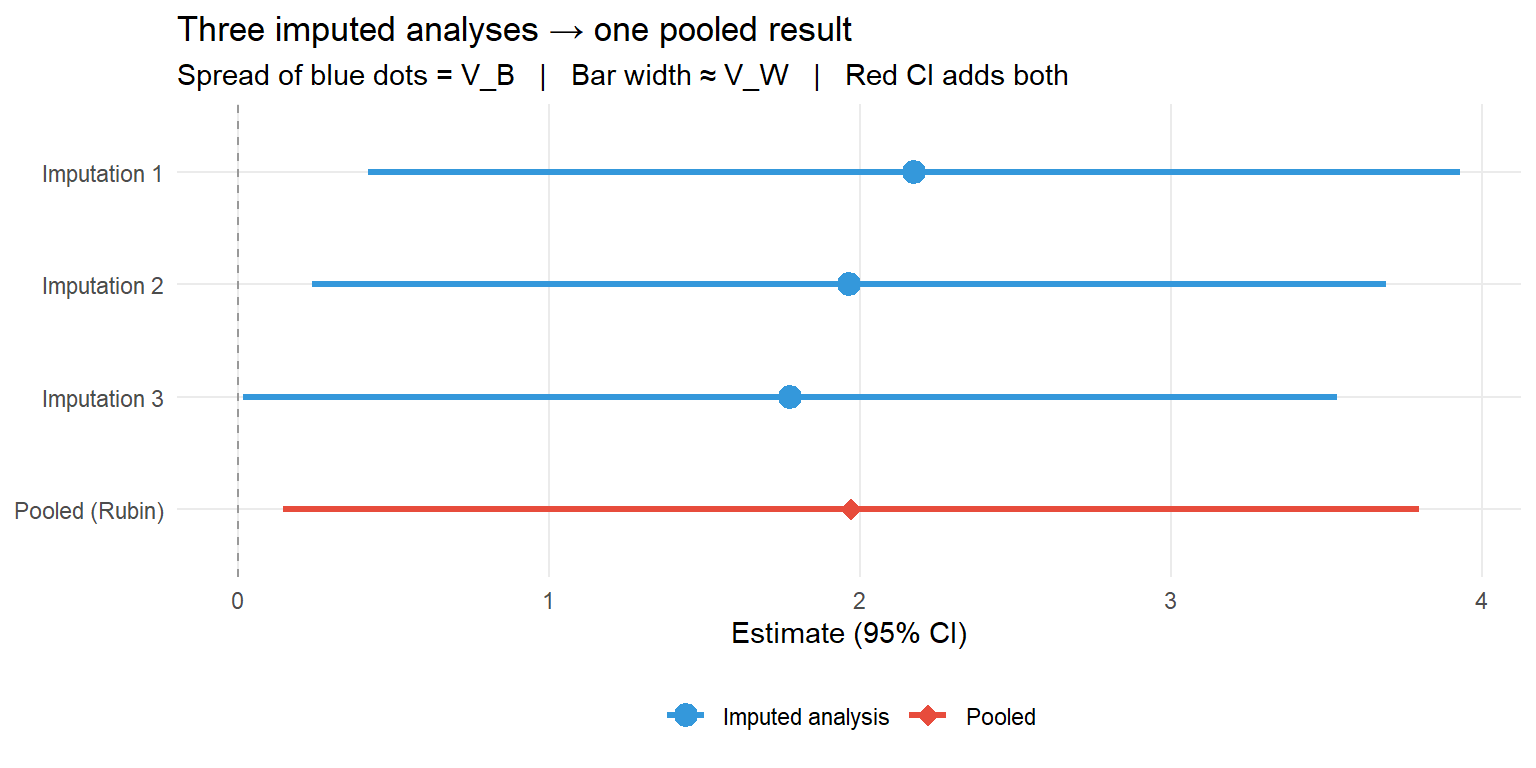
The plot below shows both sources of uncertainty. Each row is one imputed analysis: the dot is the estimate and the bar is the 95% CI. The pooled row combines both.

TipWhat to look for

The three blue dots occupy different positions — that spread is \(V_B\). The bars are similar in length — that average width is \(\sqrt{V_W}\). The pooled red bar is slightly wider than any single blue bar, because \(V_T = V_W + V_B(\text{adjusted})\) exceeds \(V_W\) alone. The extra width is the price of missing data.

1.5 Step 4 — Total variance V_T

The two components are combined with a small correction for using only M imputations rather than infinitely many (Formula 9.4):

\[V_T = V_W + V_B + \frac{V_B}{M} = V_W + \left(1 + \frac{1}{M}\right)V_B\]

For our numbers:

\[V_T = 0.7957 + 0.040 + \frac{0.040}{3} = 0.7957 + 0.040 + 0.0133 = 0.8490\]

\[SE_{pooled} = \sqrt{V_T} = \sqrt{0.8490} = 0.921\]

The \(V_B/M\) term shrinks as M grows. When M is large, \((1 + 1/M) \approx 1\) and the correction becomes negligible — one reason to prefer M = 20 or more in practice rather than the older default of M = 5.

V_T = 0.54, simply adding V_W and V_B with no correction for finite M

V_T = 0.548, adding V_W and the finite-M-adjusted between component (1 + 1/5) · V_B

V_T = 0.108, dividing the combined variance by M to average across imputations

V_T = 0.020, multiplying the within and between components as independent terms

V_T = V_W + (1 + 1/M) · V_B = 0.50 + 1.2 × 0.04 = 0.50 + 0.048 = 0.548. The factor (1 + 1/M) = 6/5 = 1.2 inflates V_B to account for using M = 5 instead of infinitely many imputations. As M → ∞, (1 + 1/M) → 1 and V_T → V_W + V_B.

1.6 Step 5 — Fraction of missing information λ

The fraction of missing information (FMI) summarises how much of the total uncertainty is due to the missingness:

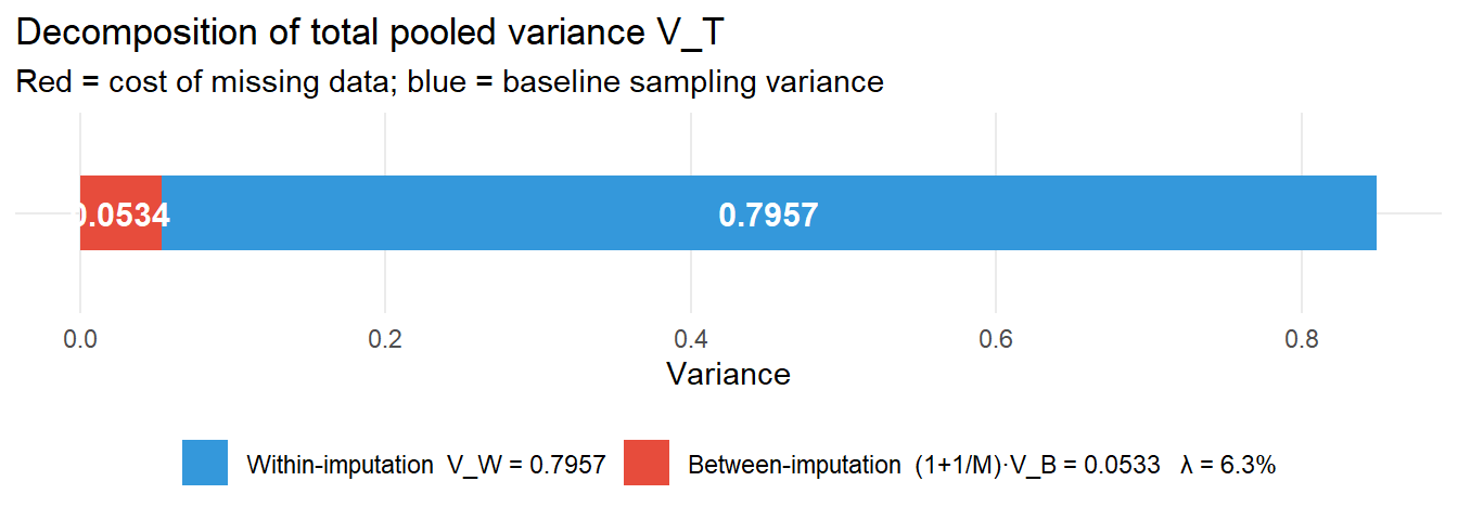
\[\lambda = \frac{(1 + 1/M)\cdot V_B}{V_T} = \frac{0.040 + 0.0133}{0.8490} = 0.063\]

\(\lambda = 0.063\) means 6% of the total variance in this estimate comes from missing data. When \(\lambda\) is small, MI and CC will agree closely; when \(\lambda\) is large (above 0.30), the missing data are heavily influencing the result and more imputations are needed.

The stacked bar below decomposes \(V_T\) visually:

Researcher A has more missing rows, since λ directly reflects the missing data proportion

Researcher A needs more imputations — high λ means between-imputation variance dominates and M = 5 is too few

Researcher B's imputation model is mis-specified since low λ signals poor predictive accuracy

Both analyses are equivalently reliable since M = 5 is the standard recommendation regardless of λ

λ is the fraction of missing information — the share of V_T attributable to missingness — not the proportion of rows missing. High λ = 0.45 means 45% of total variance comes from the imputation uncertainty. A rule of thumb: use at least 100 × λ percent imputations (so λ = 0.45 suggests M ≥ 45). For λ = 0.05, M = 5 is more than adequate. Researcher B's analysis is fine; Researcher A should increase M substantially.

1.7 Step 6 — Degrees of freedom and the confidence interval

The pooled test statistic follows a t-distribution. Rubin’s original formula for the degrees of freedom was (Formula 9.8):

\[df_{Old} = \frac{M - 1}{\lambda^2} = \frac{2}{0.063^2} = 507\]

Barnard & Rubin (1999) proposed an adjusted formula for small samples (Formula 9.9):

\[df_{Adj} = \frac{df_{Old} \cdot df_{Obs}}{df_{Old} + df_{Obs}}\]

where \(df_{Obs}\) adjusts the observed degrees of freedom \((n - k)\) by \(\lambda\) (Formula 9.10):

\[df_{Obs} = \frac{n-k+1}{n-k+3} \cdot (n-k)(1-\lambda) = \frac{149}{151} \times 148 \times 0.937 = 136.9\]

\[df_{Adj} = \frac{507 \times 136.9}{507 + 136.9} = 107.8\]

The mice package uses the adjusted formula. R’s pool() and SPSS differ here — SPSS uses \(df_{Old}\), producing a larger df and a slightly smaller p-value. The 95% CI is (Formula 9.11):

\[\bar{\theta} \pm t_{df_{Adj},\,0.975} \times SE_{pooled} = 1.971 \pm 1.982 \times 0.921 = (0.15,\; 3.79)\]

---

2 Worked Example: MI on a Simulated Cohort

A cohort of n = 150 patients receives control or treatment, age is recorded, and systolic blood pressure (SBP) is measured at follow-up. Older patients (age > 60) have a 30% probability of missing the follow-up measurement; younger patients 15%. Missingness depends on observed age — a MAR mechanism.

2.1 Explore the missing data

cat("Total rows:", nrow(dat), "\n")

Total rows: 150 

cat("Missing SBP:", sum(is.na(dat$sbp)),
    " (", round(mean(is.na(dat$sbp)) * 100), "%)\n\n")

Missing SBP: 22  ( 15 %)

# Is age associated with missingness?
t.test(age ~ is.na(sbp), data = dat)

    Welch Two Sample t-test

data:  age by is.na(sbp)
t = -1.785, df = 26.778, p-value = 0.0856
alternative hypothesis: true difference in means between group FALSE and group TRUE is not equal to 0
95 percent confidence interval:
 -9.1825696  0.6403821
sample estimates:
mean in group FALSE  mean in group TRUE 
           54.12891            58.40000 

Age is significantly higher among those with missing SBP — confirming the MAR pattern. Complete case analysis would systematically under-represent older patients.

2.2 Run mice

imp <- mice(dat[, c("sbp", "group", "age")],
            m = 5, method = "pmm", seed = 42, printFlag = FALSE)
imp

Class: mids
Number of multiple imputations:  5 
Imputation methods:
  sbp group   age 
"pmm"    ""    "" 
PredictorMatrix:
      sbp group age
sbp     0     1   1
group   1     0   1
age     1     1   0

mice uses predictive mean matching (pmm) — for each missing value it draws a plausible observed value from the donors whose predicted value is closest. Age and group are used as predictors for the missing SBP.

2.3 Analyse and pool

fits   <- with(imp, lm(sbp ~ group + age))
pooled <- pool(fits)
summary(pooled, conf.int = TRUE)

            term    estimate  std.error statistic       df      p.value
1    (Intercept) 106.5864498 2.33445482 45.657962 26.18058 1.718011e-26
2 groupTreatment  -5.5147440 0.81743910 -6.746367 22.48094 7.891332e-07
3            age   0.2470007 0.04267344  5.788161 22.80351 6.979910e-06
        2.5 %      97.5 %    conf.low   conf.high
1 101.7895195 111.3833801 101.7895195 111.3833801
2  -7.2079086  -3.8215793  -7.2079086  -3.8215793
3   0.1586819   0.3353195   0.1586819   0.3353195

The groupTreatment row is the primary quantity of interest: the pooled treatment effect, its pooled SE, the Barnard-Rubin degrees of freedom, the p-value, and the 95% CI.

2.4 Verify the formulas by hand

fit_list <- lapply(1:5, function(i) lm(sbp ~ group + age, data = complete(imp, i)))
ests <- sapply(fit_list, function(f) coef(f)["groupTreatment"])
ses  <- sapply(fit_list, function(f)
  summary(f)$coefficients["groupTreatment", "Std. Error"])

cat("Estimates per imputation:", round(ests, 3), "\n")

Estimates per imputation: -5.415 -5.345 -5.027 -5.538 -6.249 

cat("SEs per imputation:      ", round(ses, 3), "\n\n")

SEs per imputation:       0.637 0.646 0.657 0.655 0.658 

M     <- 5
Q_bar <- mean(ests)
V_W   <- mean(ses^2)
V_B   <- var(ests)
V_T   <- V_W + (1 + 1/M) * V_B
SE_p  <- sqrt(V_T)
lam   <- (1 + 1/M) * V_B / V_T

cat("Pooled estimate Q_bar: ", round(Q_bar, 4), "\n")

Pooled estimate Q_bar:  -5.5147 

cat("Within variance V_W:   ", round(V_W,   4), "\n")

Within variance V_W:    0.4232 

cat("Between variance V_B:  ", round(V_B,   4), "\n")

Between variance V_B:   0.2041 

cat("Total variance V_T:    ", round(V_T,   4), "\n")

Total variance V_T:     0.6682 

cat("SE_pooled:             ", round(SE_p,  4), "\n")

SE_pooled:              0.8174 

cat("FMI lambda:            ", round(lam,   4), "\n")

FMI lambda:             0.3666 

These values match summary(pool(fits)) — the pooled estimate, SE, and FMI are identical.

2.5 Compare to complete case

fit_cc <- lm(sbp ~ group + age, data = dat[!is.na(dat$sbp), ])
cc_est <- coef(fit_cc)["groupTreatment"]
cc_se  <- summary(fit_cc)$coefficients["groupTreatment", "Std. Error"]

cat("Complete case:  estimate =", round(cc_est, 3), "  SE =", round(cc_se, 3), "\n")

Complete case:  estimate = -5.647   SE = 0.712 

cat("Pooled (MI):    estimate =", round(Q_bar,  3), "  SE =", round(SE_p, 3), "\n")

Pooled (MI):    estimate = -5.515   SE = 0.817 

Under MAR with age included in both the imputation model and the analysis, the estimates are similar. The MI standard error is smaller — it recovers information from the rows that had missing SBP but observed age and group.

---

3 Guided Practice

Compute Rubin’s rules by hand for M = 5 imputations. The numbers are given; apply the formulas step by step.

R is loading — exercises become interactive once the status bar disappears.

TipHints

• Task 1: mean(ests)
• Task 2: V_W <- mean(ses^2) and V_B <- var(ests)
• Task 3: V_T <- V_W + (1 + 1/M) * V_B; SE_p <- sqrt(V_T); lambda <- (1 + 1/M) * V_B / V_T
• Task 4: qt(0.975, df = 50) ≈ 2.009; CI = Q_bar ± qt(0.975, 50) * SE_p

---

4 Retrieval Challenge

NoteModel answer

M      <- 10
Q_bar  <- mean(ests_ch)                        # 0.839
V_W    <- mean(ses_ch^2)                       # 0.0530
V_B    <- var(ests_ch)                         # 0.00268
V_T    <- V_W + (1 + 1/M) * V_B               # 0.0559
SE_p   <- sqrt(V_T)                            # 0.2365
lambda <- (1 + 1/M) * V_B / V_T               # 0.0527

df_old <- (M - 1) / lambda^2                   # 3241
df_obs <- ((n-k+1)/(n-k+3)) * (n-k) * (1 - lambda)  # 71.1
df_adj <- df_old * df_obs / (df_old + df_obs)  # 70.0

t_val  <- Q_bar / SE_p                         # 3.55
p_val  <- 2 * pt(-abs(t_val), df = df_adj)     # 0.001
ci_lo  <- Q_bar - qt(0.975, df_adj) * SE_p     # 0.37
ci_hi  <- Q_bar + qt(0.975, df_adj) * SE_p     # 1.31

cat("Q_bar =", round(Q_bar, 3), " SE =", round(SE_p, 3),
    "\n95% CI: (", round(ci_lo, 3), ",", round(ci_hi, 3), ")",
    "\np-value:", round(p_val, 4))

With λ = 0.053, missing data account for only 5% of total variance — M = 10 is more than adequate here.

---

5 Why-Questions

CautionQ: “Can I just use complete case analysis if age (the cause of missingness) is in my model?”

Under MAR, yes — if the variable driving missingness is included as a covariate, CC is unbiased. The worked example shows this: both CC and MI give similar estimates because age is in both the imputation model and the regression.

The advantage of MI is efficiency: MI uses all n observations (with imputed outcomes) rather than only the complete cases, reducing the SE. The gain is roughly proportional to the fraction missing and \(\lambda\). With 25% missing and \(\lambda = 0.10\), MI gives about an 8% narrower CI. With 40% missing and \(\lambda = 0.30\), the gain becomes substantial.

CC also fails when MAR is violated — when the missingness variable is the outcome itself. Dropping missing SBP rows biases the mean of SBP even after conditioning on age, because the conditional distribution changes.

CautionQ: “Why not just impute once and analyse that single complete dataset?”

Single imputation treats the imputed values as if they were observed data — the SE from the single complete analysis does not account for the uncertainty in those imputed values. The resulting CI is too narrow and the p-value too small.

Multiple imputation with M datasets quantifies this extra uncertainty through \(V_B\): the more the M estimates vary, the wider the pooled CI. With a single imputation, \(V_B\) is undefined (you cannot compute the variance of one number), so the between-imputation uncertainty is silently dropped. The analysis looks like a complete dataset when it is not.

CautionQ: “Rubin’s rules pool regression coefficients — can they pool anything else?”

Rubin’s rules apply to any quantity that is approximately normally distributed in large samples: regression coefficients, mean differences, and log odds ratios all qualify directly.

Quantities that are not normally distributed need transformation first:

• Odds ratios: pool on the log scale (log OR), then exponentiate the pooled estimate and CI back
• Correlation coefficients: apply Fisher’s z-transformation (\(z = \tanh^{-1}(r)\)), pool on z, then transform back
• Proportions: pool on the logit scale

The mice package handles this automatically for standard model classes — with(imp, glm(..., family = binomial)) followed by pool() pools log odds ratios internally. Manual transformation is only needed for derived quantities computed outside a model (for example, a predicted probability computed from a linear combination of pooled coefficients).

---

6 Spaced Review

NoteReview answers

Spaced review 1: \[V_T = V_W + \left(1 + \frac{1}{M}\right) V_B\]

Only the \((1 + 1/M)V_B\) term changes with M: - M = 5: \(V_T = 0.60 + 1.20 \times 0.08 = 0.696\) - M = 10: \(V_T = 0.60 + 1.10 \times 0.08 = 0.688\)

The reduction here is small (0.008) because \(V_B\) is modest relative to \(V_W\). When \(\lambda\) is high, the between component dominates and doubling M has a larger effect.

Spaced review 2:

1. MCAR — sensor failure is random, unrelated to the glucose level or any other measured variable. CC is valid.
2. MAR — dropout depends on PHQ-9, which is observed and included in the imputation model. MI under MAR is valid.
3. MNAR — whether the patient attends depends on their current pain score, which is the missing value. Neither CC nor standard MI is guaranteed unbiased; sensitivity analyses are required.

---

NoteSection summary

Quantity	Formula	Meaning
\(\bar{\theta}\)	\(\tfrac{1}{M}\sum \hat{\theta}_i\)	Pooled point estimate
\(V_W\)	\(\tfrac{1}{M}\sum SE_i^2\)	Typical within-dataset variance
\(V_B\)	\(\tfrac{1}{M-1}\sum(\hat{\theta}_i - \bar{\theta})^2\)	Extra variance from missing data
\(V_T\)	\(V_W + (1 + \tfrac{1}{M})V_B\)	Total pooled variance
\(\lambda\)	\((1+\tfrac{1}{M})V_B\;/\;V_T\)	Fraction of missing information
95% CI	\(\bar{\theta} \pm t_{df_{Adj}} \cdot \sqrt{V_T}\)	Pooled confidence interval

mice workflow in R:

imp    <- mice(dat, m = 20, method = "pmm", seed = 42)
fits   <- with(imp, lm(y ~ x1 + x2))
pooled <- pool(fits)
summary(pooled, conf.int = TRUE)

NoteFurther reading

Heymans, M.W. & Eekhout, I. (2024). Applied Missing Data Analysis with SPSS and R Studio. bookdown.org/mwheymans/bookmi/ — Chapter 9 for Rubin’s rules with full numerical examples.

van Buuren, S. (2018). Flexible Imputation of Missing Data (2nd ed.). Chapman & Hall/CRC. stefvanbuuren.name/fimd/ — Chapters 2–4 for theory, Chapter 5 for the mice workflow.