CS1.5 — Inference & Diagnostics

1 Before You Start

Recall: the random intercept model

The model in this chapter is Y_ij = β₀ + β₁·treat + β₂·dbp1 + b_i + ε_ij, where:

β₀, β₁, β₂ are fixed effects — the same for every centre
b_i ~ N(0, σ²_b) is the random effect for centre i — how much centre i deviates from the population average
ε_ij ~ N(0, σ²) is the residual for patient j in centre i

If any of these is unclear, revisit CS1.2 before continuing.

Recall: REML vs ML

REML is the default in lme4 and gives unbiased variance component estimates. Use ML (REML=FALSE) only when comparing models with different fixed effects via LRT. For comparing random effects structures, REML is approximately correct.

Revisit CS1.3 if this distinction is uncertain.

Recall: likelihood ratio test (LRT)

The LRT statistic is Λ = −2·(ℓ_restricted − ℓ_full). Under H₀, Λ ~ χ²(df), where df = difference in number of parameters. A small p-value means the additional parameters significantly improve fit.

2 Concept: Inference in Mixed Models

2.1 Hypothesis tests for fixed effects

The fixed effects in a mixed model have asymptotically normal estimators:

\[\hat{\boldsymbol{\beta}} \overset{a}{\sim} \mathcal{N}(\boldsymbol{\beta},\ (\mathbf{X}^\top \hat{\mathbf{V}}^{-1} \mathbf{X})^{-1})\]

This gives Wald $t$-statistics: $t = \hat{\beta}_k / \widehat{SE}(\hat{\beta}_k)$. But what degrees of freedom?

Unlike ordinary regression, there is no exact df for the $t$-test in a mixed model. Three common solutions:

Method	df	Notes
Wald $z$-test	$\infty$ (normal)	Anti-conservative in small samples
Satterthwaite	Approximate, data-dependent	Default in `lmerTest`
Kenward-Roger	Approximate, adjusted SEs	More conservative, preferred for small $m$
LRT	$\chi^2$ with df = number of constraints	Valid when using ML; preferred for multi-parameter tests

The model failed to converge — results are unreliable and should be discarded

Two fixed effect predictors are perfectly collinear

A variance component or random effects correlation is estimated at its boundary (0 or ±1)

The random effects and residuals are correlated, violating model assumptions

Singular fits most often mean a random effect explains near-zero variance (estimated at 0) or a correlation hits ±1. The model converged, but the random effects structure may be overparameterised relative to the data. Consider simplifying: remove a random slope, or constrain the correlation to zero.

2.2 Confidence intervals

Three methods for CIs on fixed effects:

Wald: $\hat{\beta}_k \pm z_{0.975} \cdot \widehat{SE}(\hat{\beta}_k)$ — fast, assumes normality
Profile likelihood: trace the likelihood; more accurate, especially for small samples
Parametric bootstrap: simulate data under the fitted model, refit; most accurate but slow

# Wald CI (manual)
beta   <- fixef(fit)["treatTreatment"]
se     <- sqrt(diag(vcov(fit)))["treatTreatment"]
wald_ci <- c(beta - 1.96*se, beta + 1.96*se)

# Profile likelihood CI
prof_ci <- confint(fit, parm="treatTreatment", method="profile")

Computing profile confidence intervals ...

cat("Wald CI:   ", round(wald_ci, 3), "\n")

Wald CI:    -3.641 -2.184

cat("Profile CI:", round(prof_ci, 3), "\n")

Profile CI: -3.641 -2.185

Compare the BLUP estimates from both models using a t-test, since BLUPs capture the random effects information most directly

Compare adjusted R² values between the two models, since R² accounts for random effects variance and is the standard criterion

Use AIC only — an LRT is not valid for comparing random effects structures because it requires equal fixed effects between models

Use a likelihood ratio test, but note that the p-value is conservative because σ²=0 is on the boundary of the parameter space

Testing H₀: σ²_slope = 0 is a boundary test — the null is at the edge of the valid parameter space. This makes the standard χ² approximation for the LRT conservative (p-value too large). A common correction is to halve the p-value. AIC is a reasonable alternative that does not have this issue.

2.3 Assumptions

The linear mixed model makes four key assumptions:

Linearity: $E[Y_{ij} | \mathbf{x}_{ij}, b_i] = \mathbf{x}_{ij}^\top \boldsymbol{\beta} + b_i$
Normality of random effects: $b_i \sim \mathcal{N}(0, \sigma_b^2)$
Normality of residuals: $\varepsilon_{ij} \sim \mathcal{N}(0, \sigma^2)$
Independence: $b_i \perp \varepsilon_{ij}$, and $b_i \perp \mathbf{x}_{ij}$ (exogeneity)

Which assumption matters most?

Exogeneity ($b_i \perp \mathbf{x}_{ij}$) is the most consequential. Violation biases $\hat{\boldsymbol{\beta}}$ — use the Hausman test or fixed effects if suspected.
Normality of $b_i$ is less important for fixed effects inference (CLT applies), but matters for BLUP prediction.
Normality of $\varepsilon_{ij}$ can be checked via residual plots; mild violations are tolerable.
Linearity should always be examined via residual vs fitted plots.

The fixed effect estimates are biased — heavy tails in random effects introduce systematic error in the slope and intercept estimates

The ICC is severely underestimated because heavy-tailed random effects inflate the between-cluster variance beyond the model's estimate

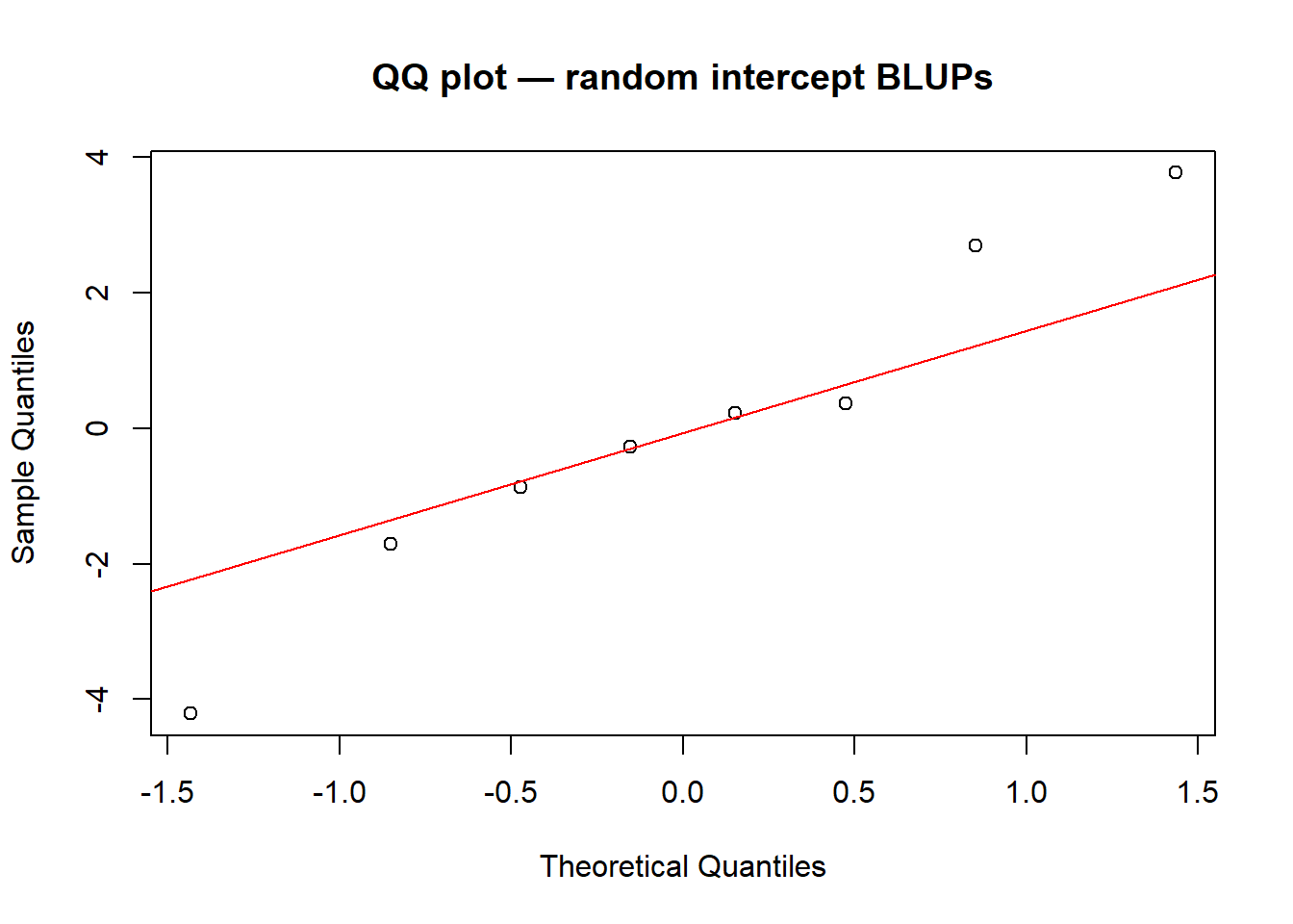
The normality assumption for b_i ~ N(0, σ²_b) may be violated — the random effects distribution has heavier tails than assumed

The model needs additional fixed effect predictors — heavy tails indicate unexplained systematic variation in the response variable

Mixed models assume b_i ~ N(0, σ²_b). Heavy tails or skewness in the Q-Q plot of random effects suggest this assumption is questionable. With many groups (>30), fixed effect estimates are fairly robust to mild violations, but inference on variance components can be affected.

2.4 Broad and Narrow Inference

A mixed model can answer two quite different questions, depending on which population you want to draw conclusions about.

	Broad inference	Narrow inference
Question	What is the treatment effect in a new, randomly selected centre?	What happened in these specific centres in this study?
Answers via	Fixed effects β	BLUPs b̂_i
Scope	Population of all possible centres	Only the centres actually observed

Fixed effects (β) answer the broad inference question. β₁ estimates the average treatment effect you would expect if a new centre were drawn from the same population of centres.

BLUPs (Best Linear Unbiased Predictors) answer the narrow inference question. b̂_i is the predicted value of the random effect for centre i — how much that specific centre deviates from the population mean, after accounting for fixed effects. In R: ranef(fit)$center.

2.4.1 Shrinkage: why BLUPs are not just raw group means

BLUPs do not simply use each centre’s observed mean. Instead, they shrink toward zero — the extent depending on how much information that centre provides:

Centres with few patients → more shrinkage (less data → rely more on the population average)
Centres with many patients → less shrinkage (more data → trust the observed centre mean more)
High ICC → less shrinkage overall (between-centre variation is large and well-estimated)

This is a desirable property: shrinkage reduces overfitting and gives better predictions for new patients at that centre.

Reading the shrinkage plot

Every point below the dashed diagonal is a centre whose BLUP has been pulled toward zero compared to its raw mean. Points near the red dotted line (zero) have been shrunk the most. Smaller dots (fewer patients) tend to sit further below the diagonal — exactly as the shrinkage formula predicts.

Narrow inference — answered by BLUPs

Broad inference — answered by the fixed effect β

A within-cluster contrast — not estimable from this model

A random effects prediction — answered by ranef()

Broad inference asks about the population of all possible groups (hospitals, centres, etc.), not just those in the study. The fixed effect β₁ gives the expected treatment effect averaged over that population. BLUPs (narrow inference) describe the specific hospitals in this study only.

3 Worked Example: Diagnostic Plots

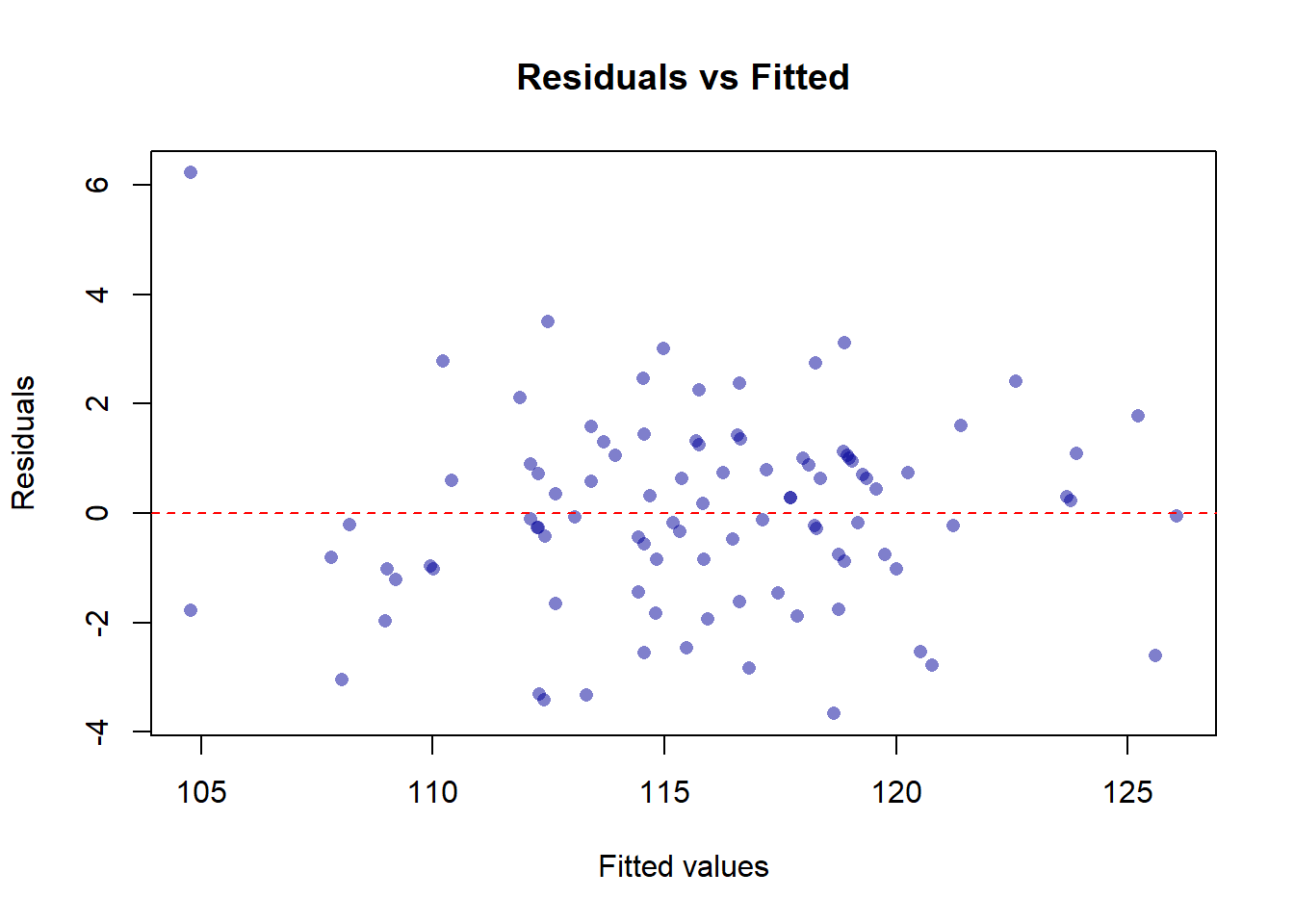
# Residuals vs fitted
plot(fitted(fit), residuals(fit),
     xlab="Fitted values", ylab="Residuals",
     main="Residuals vs Fitted",
     pch=16, col=rgb(0,0,0.6,0.5))
abline(h=0, lty=2, col="red")

Points scattered randomly around the horizontal zero line with roughly constant spread

A fan shape — spread of residuals increases (or decreases) with the fitted value

Points centred slightly above zero for a few fitted values

A small number of points with large residuals, otherwise random

A fan shape indicates heteroscedasticity — the residual variance is not constant (it depends on the fitted value), violating the assumption ε_ij ~ N(0, σ²). Random scatter around zero with roughly constant width is what you want to see. A curved pattern (bow shape) would indicate a linearity violation instead.

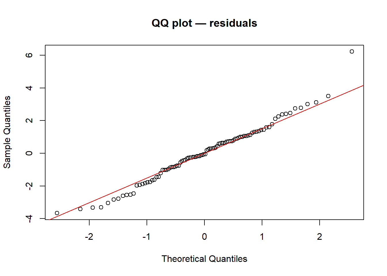
# QQ plot of residuals
qqnorm(residuals(fit), main="QQ plot — residuals")
qqline(residuals(fit), col="red")

The random effects b_i are not normally distributed — this Q-Q plot is where you check that assumption rather than examining ε_ij

The within-cluster residuals have heavier tails than the normal — extreme deviations from the model fit occur more often than expected

The fixed-effect estimates β̂ are biased — heavy tails in residuals introduce systematic error that becomes more severe with larger samples

There is multicollinearity among the predictors — correlated fixed effects produce heavy-tailed residuals as a known consequence

Heavy tails in the Q-Q plot mean some residuals are much larger (or smaller) than a normal distribution would predict. This is a violation of the normality assumption for ε_ij. Mild violations are tolerable, especially with large n (CLT). The Q-Q plot of BLUPs (ranef) is a separate check for b_i normality.

# QQ plot of BLUPs (check normality of random effects)
blups <- ranef(fit)$center[,1]
qqnorm(blups, main="QQ plot — random intercept BLUPs")
qqline(blups, col="red")

# Satterthwaite degrees of freedom via lmerTest
# Note: lmerTest re-exports lmer with df approximation built in
library(lmerTest)


Attaching package: 'lmerTest'

The following object is masked from 'package:lme4':

    lmer

The following object is masked from 'package:stats':

    step

fit_t <- lmer(dbp ~ treat + dbp1 + (1|center), data=dat, REML=TRUE)
summary(fit_t)  # now shows df and p-values

Linear mixed model fit by REML. t-tests use Satterthwaite's method [
lmerModLmerTest]
Formula: dbp ~ treat + dbp1 + (1 | center)
   Data: dat

REML criterion at convergence: 414

Scaled residuals: 
    Min      1Q  Median      3Q     Max 
-2.0144 -0.5577 -0.0356  0.5597  3.4241 

Random effects:
 Groups   Name        Variance Std.Dev.
 center   (Intercept) 6.435    2.537   
 Residual             3.304    1.818   
Number of obs: 96, groups:  center, 8

Fixed effects:
               Estimate Std. Error       df t value Pr(>|t|)    
(Intercept)    82.88300    2.19974 81.46169  37.678  < 2e-16 ***
treatTreatment -2.91250    0.37162 86.00215  -7.837 1.13e-11 ***
dbp1            0.38181    0.02218 86.25132  17.216  < 2e-16 ***
---
Signif. codes:  0 '***' 0.001 '**' 0.01 '*' 0.05 '.' 0.1 ' ' 1

Correlation of Fixed Effects:
            (Intr) trtTrt
treatTrtmnt -0.035       
dbp1        -0.905 -0.055

Fixed effects:
                  Estimate Std. Error       df t value Pr(>|t|)
(Intercept)         45.32       8.14    6.001    5.57  0.00148 **
treatTreatment      -3.18       2.41    5.998   -1.32  0.23456
dbp1                 0.38       0.09   85.012    4.22  5.1e-05 ***

treatTreatment has fewer unique values than dbp1, so the Satterthwaite approximation assigns it fewer effective degrees of freedom by design

Treatment is assigned at the centre level (between-cluster), so effective df ≈ number of centres; dbp1 varies within centres, drawing on all patients

Satterthwaite always assigns fewer df to categorical predictors than to continuous ones because binary contrasts carry less information

dbp1 is a continuous predictor and continuous variables always receive more degrees of freedom than categorical ones in any linear mixed model

The Satterthwaite approximation allocates df based on where the predictor varies. Treatment is a between-cluster predictor (all patients in a centre get the same treatment) — the comparison has only m = 8 centres as independent units, giving df ≈ 6 (centres minus 2 fixed effects). dbp1 varies patient-by-patient within centres, drawing on the full n = 96 observations, giving df ≈ 85. Low df for between-cluster predictors means wider CIs and larger p-values — reflecting genuine uncertainty.

4 Guided Practice

R is loading in the background — the exercises below will be interactive once the status bar disappears. You can read the concept sections above immediately.

Hints

residuals(fit_sk) for residuals
ranef(fit_sk)$group[,1] for BLUPs
Compare fixef(fit_sk) to true values

5 Retrieval Challenge

Model answers

Q1: Fan shape → heteroscedasticity (non-constant variance). Try a log or square root transformation of $Y$, or use a variance function (e.g., nlme::lme with weights = varPower()).

Q2: Two BLUPs as outliers out of $m$ groups suggests possible influential groups, not a systematic failure. Check whether those groups are unusual in the data. Fixed effects are more robust to BLUP outliers than to residual outliers.

Q3: If a predictor varies only between groups and is correlated with the random effect, the model is mis-specified — the random effect “absorbs” some of the predictor’s variance, biasing its coefficient. The output above shows income is estimated far from 0.8 because of this confounding. This is the classic “within vs between” problem in panel data.

6 Why-Questions

Q: “lmerTest gives a different p-value than the z-test from the default summary. Which is correct?”

Neither is exact. The z-test (Wald with normal distribution) treats the $t$-statistic as if df = ∞. lmerTest’s Satterthwaite approximation computes data-dependent approximate df. With large $m$ (many groups) and large $n_i$, both converge.

With small $m$ (e.g., 8 centres), the Satterthwaite or Kenward-Roger approximation is more accurate. The z-test p-values are anti-conservative (too small). Use lmerTest for final reporting when in doubt.

Q: “Profile likelihood CIs are different from Wald CIs. How big a difference matters?”

As a rule of thumb: if the absolute difference exceeds 10% of the CI width, profile likelihood is materially more accurate and should be preferred. This tends to happen when:

$m$ is small (< 20 groups)
The variance component is near 0 (the likelihood is asymmetric near the boundary)
The sample size per group is unbalanced

Profile CIs take longer to compute (lme4 uses numerical optimisation to trace the likelihood contour) but are standard practice in published work.

7 Spaced Review

Review answer

\[\text{ICC} = \frac{\hat{\sigma}_b^2}{\hat{\sigma}_b^2 + \hat{\sigma}^2} = \frac{\texttt{vc\$vcov[1]}}{\texttt{vc\$vcov[1] + vc\$vcov[2]}}\]