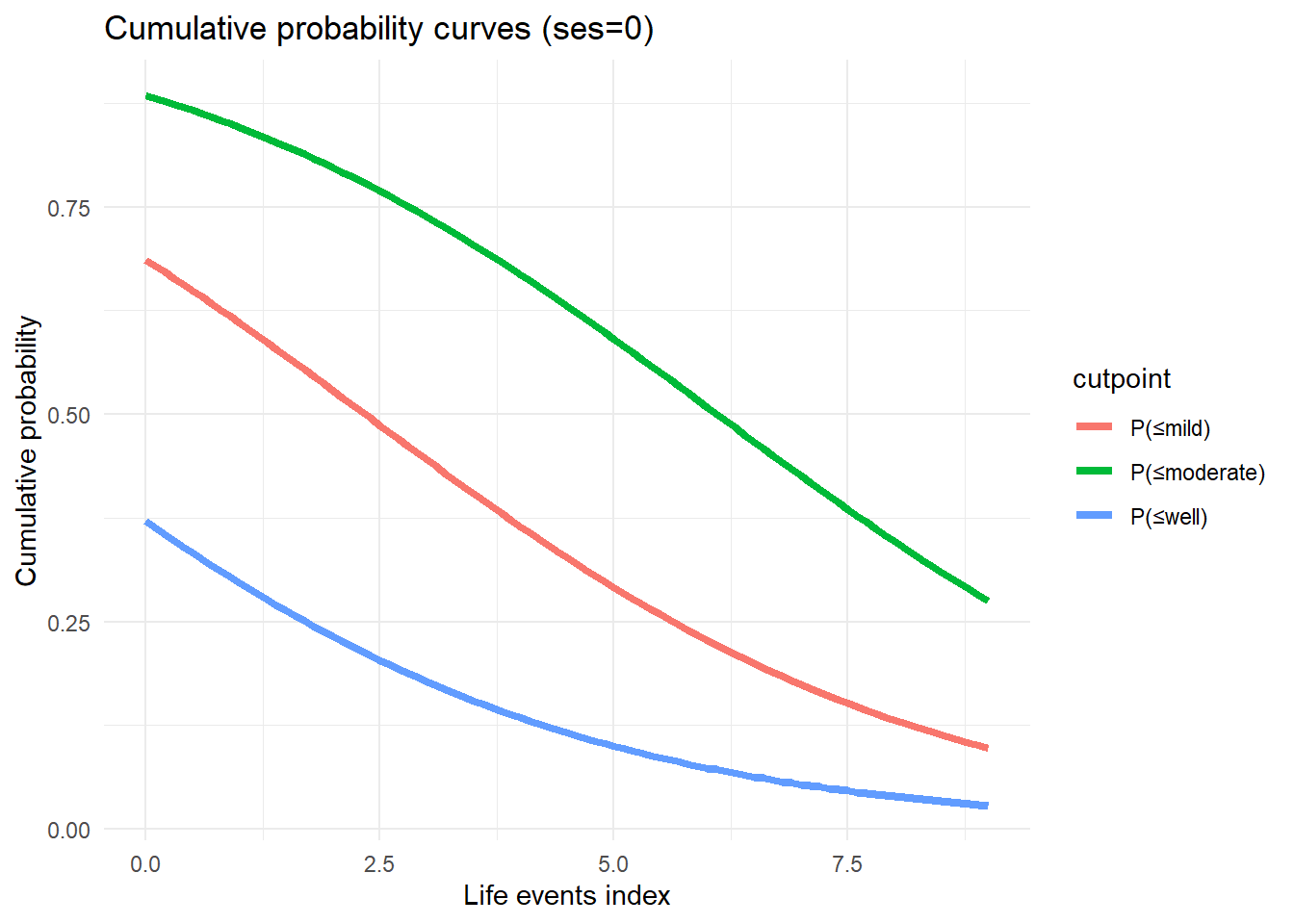
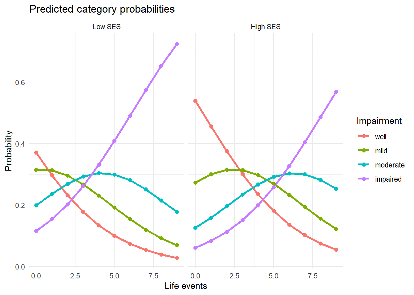
The proportional odds (PO) model — also called the cumulative logit model or cumulative link model (CLM) — is the standard approach for ordinal outcomes. Rather than modelling the probability of each category separately, it models the probability of being at or below each category: P(Y ≤ 1), P(Y ≤ 2), and so on. These are called cumulative probabilities.
Each cumulative probability is modelled with a logistic equation that shares the same predictor coefficients but has its own intercept (called a threshold or cutpoint). This single set of coefficients is what makes the model parsimonious: one odds ratio (OR) per predictor summarises its effect across all category boundaries simultaneously.
The key assumption is proportional odds: the OR for any predictor is the same regardless of which cumulative split you look at. Geometrically, this means the logistic curves for each cumulative probability are parallel — they differ only by horizontal shifts. This assumption can be tested, and CS3.3 covers what to do when it fails.
On this page you will learn how the cumulative logit is defined, how to read and interpret polr() output, and how to compute odds ratios from the coefficient table.
NoteAbbreviations used on this page
Abbreviation
Full term
PO
Proportional odds
CLM
Cumulative link model
OR
Odds ratio
CI
Confidence interval
MLE
Maximum likelihood estimator
1 Concept: The Cumulative Logit and Proportional Odds
1.1 Cumulative probabilities
Instead of modelling individual category probabilities \(P(Y = k)\), the cumulative logit model uses cumulative probabilities:
\[P(Y \leq k | \mathbf{x}) = F(\alpha_k - \mathbf{x}^\top\boldsymbol{\beta})\]
The model has: - \(K-1\)thresholds\(\alpha_1 < \alpha_2 < \cdots < \alpha_{K-1}\) - A single coefficient vector \(\boldsymbol{\beta}\) — shared across all cumulative equations
4 — one per category
3 — one for each of the K−1 cumulative splits
1 — the PO assumption collapses all thresholds into one
It depends on the number of predictors
The model has K−1 = 3 thresholds (α₁ < α₂ < α₃) defining the three cumulative binary splits: Y ≤ 1 vs Y > 1, Y ≤ 2 vs Y > 2, Y ≤ 3 vs Y > 3. These are the intercepts in polr output. The constraint α₁ < α₂ < α₃ is enforced during estimation to ensure valid probabilities.
1.2 The Proportional Odds (PO) assumption
The model implies that the log-OR for any predictor \(x_j\) is the same regardless of cut-point \(k\):
\[\log \frac{P(Y \leq k | x_j+1) / P(Y > k | x_j+1)}{P(Y \leq k | x_j) / P(Y > k | x_j)} = -\beta_j \quad \forall k\]
This is the proportional odds assumption: the odds ratio for \(x_j\) is constant across all binary splits of the outcome. On the logit scale, the regression lines for each cut-point are parallel.
The probability of each category is proportional to the predictor value
The odds ratios for each predictor increase proportionally across categories
The log-OR for any predictor is the same regardless of which binary split of the outcome is used
The thresholds are equally spaced on the logit scale
Under PO, the effect of x on log-odds(Y ≤ k) is −β for every cut-point k. On the logit scale, the K−1 cumulative regression lines are parallel. This is what allows a single β to summarise the predictor's effect across all cumulative comparisons, making the model parsimonious.
ImportantSign convention — MASS::polr vs ordinal package
So a positive\(\beta\) means the predictor decreases the probability of being in a lower category (shifts towards higher categories).
The ordinal::clm package uses the same convention. Some software (e.g., VGAM with reverse=FALSE) uses \(\alpha_k + \boldsymbol{\beta}^\top\mathbf{x}\), reversing the sign. Always check the parameterisation before interpreting.
Higher x is associated with lower (earlier) categories — in polr, a positive coefficient increases P(Y ≤ k)
Higher x is associated with higher (later) categories — the probability of being in a lower category decreases
The coefficient has the same sign interpretation as in linear regression — positive means the response increases
The predictor violates the proportional odds assumption, making the coefficient unstable across cut-points
polr uses logit P(Y ≤ k) = α_k − β'x. A positive β means increasing x decreases logit P(Y ≤ k), which decreases P(Y ≤ k), so the response shifts towards higher categories. This sign is opposite to some other software — always check the parameterisation before interpreting. exp(β) gives the OR for Y > k vs Y ≤ k.
1.3 From cumulative probabilities to category probabilities
\[P(Y = k | \mathbf{x}) = P(Y \leq k | \mathbf{x}) - P(Y \leq k-1 | \mathbf{x})\]
with \(P(Y \leq 0) = 0\) and \(P(Y \leq K) = 1\).
2 Worked Example
library(MASS)fit <-polr(impair ~ ses + life, data=dat, Hess=TRUE)summary(fit)
Call:
polr(formula = impair ~ ses + life, data = dat, Hess = TRUE)

Coefficients:
       Value Std. Error t value
ses  -0.6870    0.26690  -2.574
life  0.3341    0.04891   6.830

Intercepts:
                  Value   Std. Error t value
well|mild         -0.5288  0.2822    -1.8740
mild|moderate      0.7822  0.2842     2.7522
moderate|impaired  2.0388  0.3150     6.4730

Residual Deviance: 489.1818
AIC: 499.1818
Reading the output: - ses, life: regression coefficients \(\boldsymbol{\beta}\) (positive = shifts towards higher categories) - well|mild, mild|moderate, moderate|impaired: thresholds \(\alpha_1, \alpha_2, \alpha_3\) - Value column: estimates; Std. Error: standard errors; t value: Wald statistic (asymptotically normal)
Coefficients:
       Value Std. Error t value
ses   -0.898     0.247  -3.636
life   0.381     0.076   5.013

Intercepts:
                   Value Std. Error t value
well|mild         -0.527      0.238  -2.215
mild|moderate      0.781      0.237   3.296
moderate|impaired  2.208      0.266   8.294
Higher SES is associated with worse impairment — the response shifts to higher (worse) categories because a negative coefficient decreases P(Y ≤ k)
Higher SES is associated with better outcomes — it increases P(Y ≤ k) for each cut-point, shifting the response towards lower (better) categories
The t value of −3.6 means the effect is not significant — conventional rules require t values above ±2 for statistical significance
The coefficient cannot be interpreted because polr does not use standard logistic regression and the sign convention differs from GLM output
In polr: logit P(Y ≤ k) = α_k − β'x. With β_ses = −0.898, we get logit P(Y ≤ k | ses=1) = α_k − (−0.898) = α_k + 0.898. This is larger than α_k, so P(Y ≤ k | ses=1) > P(Y ≤ k | ses=0) — higher SES means a higher cumulative probability of being in a lower (better) category. The OR for the response falling in a higher vs lower category: exp(β_ses) = exp(−0.898) ≈ 0.41. People with higher SES have about 41% of the odds of worse-vs-better compared to lower SES. |t| = 3.6 is well above 1.96 — the effect is significant.
# Odds ratios (note: in polr parameterisation, higher x → higher category)cat("Odds ratios (exp(coef)):\n")
Odds ratios (exp(coef)):
round(exp(coef(fit)), 4)
   ses   life
0.5031 1.3966
# Confidence intervalsci <-confint(fit) # profile likelihood by default
Waiting for profiling to be done...
round(exp(ci), 4)
      2.5 % 97.5 %
ses  0.2969 0.8464
life 1.2714 1.5406
# The same model fitted with ordinal::clm# clm uses the same parameterisation as polr: logit P(Y≤k) = α_k − β'xlibrary(ordinal)fit_clm <-clm(impair ~ ses + life, data=dat)summary(fit_clm)
formula: impair ~ ses + life
data:    dat

 link  threshold nobs logLik  AIC    niter max.grad cond.H
 logit flexible  200  -244.59 499.18 4(0)  3.48e-08 3.8e+02

Coefficients:
     Estimate Std. Error z value Pr(>|z|)
ses  -0.68704    0.26690  -2.574     0.01 *
life  0.33407    0.04891   6.830 8.49e-12 ***
---
Signif. codes:  0 '***' 0.001 '**' 0.01 '*' 0.05 '.' 0.1 ' ' 1

Threshold coefficients:
                  Estimate Std. Error z value
well|mild          -0.5288     0.2822  -1.874
mild|moderate       0.7822     0.2842   2.752
moderate|impaired   2.0388     0.3150   6.473
Notepolr vs clm: what differs?
Both packages fit the same proportional odds model with the same parameterisation (\(\text{logit}\,P(Y \leq k) = \alpha_k - \boldsymbol{\beta}^\top\mathbf{x}\)). The output looks different but the coefficients are numerically the same.
Key practical differences:
MASS::polr
ordinal::clm
Calls thresholds
$zeta
printed as intercepts
p-values
not printed (use \(z\)-test manually)
printed directly
CIs
confint() → profile likelihood
confint() → profile likelihood
PO testing
manual LRT
nominal_test() (CS3.3)
Standard errors
expected information matrix
observed information matrix
For most purposes the results are interchangeable. ordinal is preferred when you need nominal_test() or partial PO models.
# Verify: coefficients should match (up to rounding)cat("polr coefficients:\n")
The PO assumption — single \(\boldsymbol{\beta}\) — means each curve is a horizontally shifted version of the others. The shift equals \(\alpha_k - \alpha_{k-1}\). This parallelism is what we test in CS3.3.
R is loading in the background — the exercises below will be interactive once the status bar disappears. You can read the concept sections above immediately.
The log-OR for a \(\Delta x\) change in \(x_j\) is: \(-\beta_j \cdot \Delta x\) (negative sign because higher \(\beta\) increases probability of higher categories, which means it decreases cumulative probabilities \(P(Y \leq k)\)).
Q1: OR = exp(0.95) ≈ 2.59 — high SES roughly 2.6× higher odds of being in a higher impairment category.
Wait — check the sign convention! In polr, positive \(\beta\) means higher \(x\) → more likely to be in a higher category. The OR = exp(+0.95) ≈ 2.59 refers to odds of being in a higher category. Check your model’s parameterisation.
5 Why-Questions
CautionQ: “The PO model gives a single OR per predictor. But what if the effect really is different for mild vs moderate vs severe?”
If the PO assumption is violated, forcing a single OR can be misleading — it represents an average that may not apply to any specific cut-point.
Options: 1. Partial proportional odds: allow some predictors to vary across equations while constraining others 2. Non-proportional odds model (full multinomial): allows all slopes to vary — loses parsimony 3. Adjacent-category model: models log-odds of adjacent categories \(P(Y=k+1)/P(Y=k)\) — another ordinal model that relaxes PO
Test PO first (CS3.3), then decide. A mild violation with little practical consequence may not warrant the added complexity.
CautionQ: “polr gives thresholds but clm gives intercepts. Are they the same?”
In polr: output is \(\alpha_k\) in \(\text{logit}\,P(Y \leq k) = \alpha_k - \boldsymbol{\beta}\mathbf{x}\). These are called zeta.
In ordinal::clm: same parameterisation, but the output uses the term “intercept” for the thresholds. They are numerically identical (given the same sign convention).
Confusion arises if the sign on \(\boldsymbol{\beta}\) is reversed. Always verify by checking a predicted probability manually: compute \(\text{logit}\,P(Y \leq k)\) from the formula and compare to plogis() applied to the threshold minus the linear predictor.
6 Spaced Review
NoteFurther reading
Agresti, A. (2010). Analysis of Ordinal Categorical Data (2nd ed.). Wiley. — Chapter 3.