CS2.4 — Predicted Probabilities

0.1 What this page is about

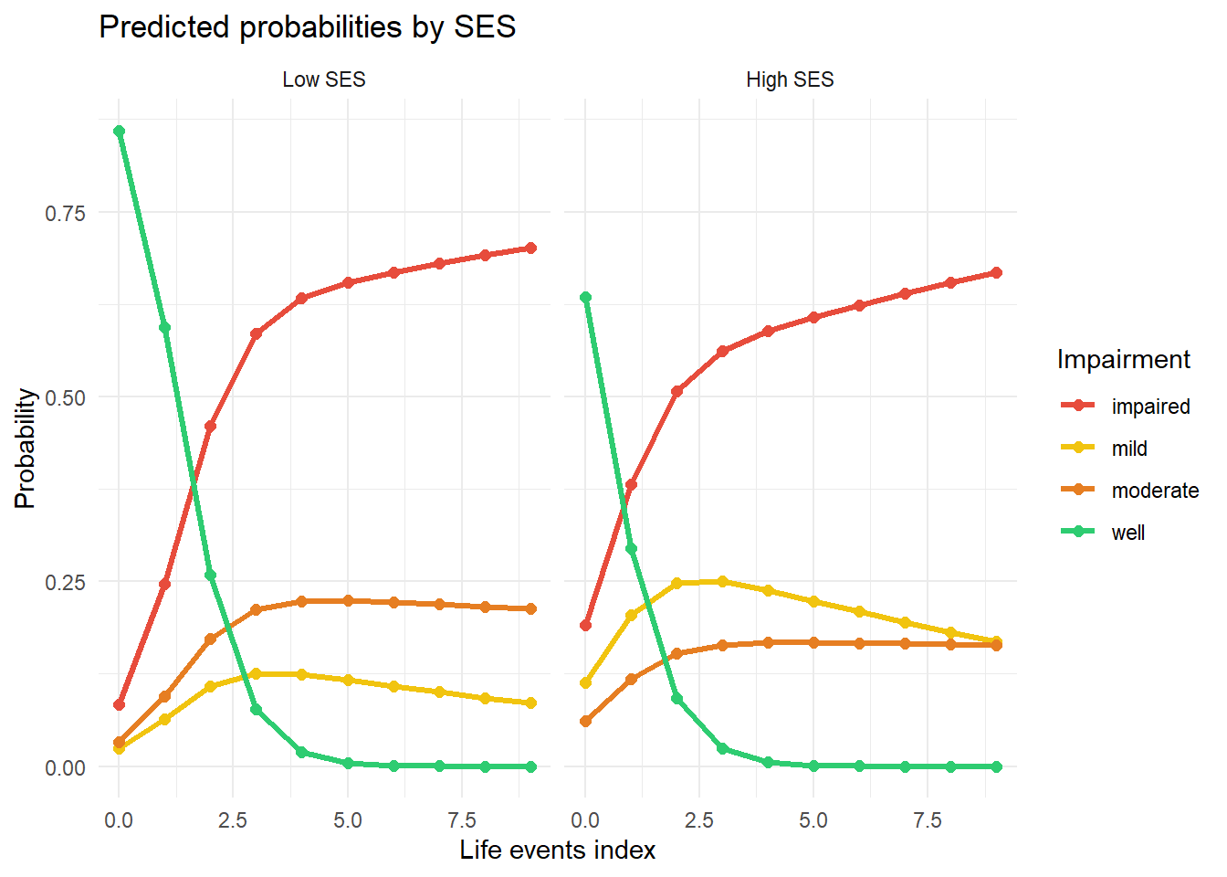
A multinomial logistic regression model produces coefficients on the log-odds scale — useful for understanding relative effects, but hard to communicate directly. If a clinician asks “what is the chance this patient ends up in the most severe category?”, you need predicted probabilities, not odds ratios (ORs).

Predicted probabilities are computed from the fitted model via the softmax function: the log-odds for each category are exponentiated and rescaled so that all category probabilities sum to 1. For any new combination of predictor values, you can obtain a complete probability distribution over all outcome categories.

A key insight is that predicted probabilities are not additive — changing one predictor shifts the entire probability distribution simultaneously, and the size of the shift depends on the current probability level. This is different from linear regression, where a coefficient directly gives the change in outcome.

On this page you will learn how to generate predicted probabilities with predict(), how to visualise how probabilities change across predictor values, and how to compare profiles of interest.

NoteAbbreviations used on this page

Abbreviation	Full term
OR	Odds ratio
MLE	Maximum likelihood estimator
SE	Standard error

---

1 Concept: From Log-Odds to Probabilities

1.1 Why probabilities, not just OR?

Odds ratios describe relative effects. For absolute risk communication (how likely is this patient to be in each category?), probabilities are more useful. The predicted probability for observation \(i\) being in category \(k\) is:

\[\hat{\pi}_{ik} = \frac{\exp(\mathbf{x}_i^\top \hat{\boldsymbol{\beta}}_k)}{1 + \sum_{j \neq r} \exp(\mathbf{x}_i^\top \hat{\boldsymbol{\beta}}_j)}\]

Key properties: - \(\hat{\pi}_{ik} \in (0,1)\) for all \(i\), \(k\) - \(\sum_k \hat{\pi}_{ik} = 1\) for all \(i\) - The effect of a predictor on \(\hat{\pi}_{ik}\) depends on the current probability level — it is non-linear

Probabilities are on a natural 0–1 scale that clinicians understand without statistical training, unlike odds ratios

Probabilities give absolute risk for a specific patient profile, while ORs only describe relative effects

Predicted probabilities are invariant to the reference category choice, unlike odds ratios which change with it

Odds ratios cannot be computed from multinomial models once the number of categories exceeds three, limiting their use

An OR of 3 for "impaired vs well" is hard to interpret without knowing baseline risk. If the baseline probability of being impaired is 1%, OR=3 means 3% risk — probably negligible. Predicted probabilities for a specific patient profile give absolute numbers that clinicians can act on.

1.2 Uncertainty in predicted probabilities

The delta method approximates the variance of \(\hat{\pi}_{ik}\):

\[\widehat{\text{Var}}(\hat{\pi}_{ik}) \approx \left(\frac{\partial \pi_{ik}}{\partial \boldsymbol{\beta}}\right)^\top \mathcal{I}^{-1} \left(\frac{\partial \pi_{ik}}{\partial \boldsymbol{\beta}}\right)\]

This gives SE for each predicted probability, enabling confidence intervals. The bootstrap is an alternative that avoids the derivative calculation.

Always equal to exp(β_k) − 1, the OR minus one, since softmax and logit are linked by exponentiation

Constant across all values of x, like in linear regression — the log-OR is constant so the probability effect must be too

Non-constant — it depends on the current probability level through the softmax function

Zero, because probabilities must sum to 1, meaning an increase in one category must cancel another

The softmax function is nonlinear, so marginal effects on probabilities depend on where you are in the probability space. A predictor's effect on π̂_k is largest when π̂_k ≈ 0.5 and smaller near 0 or 1. This is a fundamental difference from linear regression and means "average marginal effects" should be computed and reported.

A large bootstrap sample to approximate the distribution of predicted probabilities empirically

The observed residuals and a variance estimate of the residuals from the fitted multinomial model

The gradient of the predicted probability with respect to β, and the estimated covariance matrix of β̂

The assumption that predicted probabilities are normally distributed around the true probability values

The delta method approximates Var(g(β̂)) ≈ (∂g/∂β)'·Var(β̂)·(∂g/∂β), where g(β) is the predicted probability and Var(β̂) = I(β̂)⁻¹. It propagates parameter uncertainty through the nonlinear softmax transformation. It is fast but relies on the normal approximation for β̂.

---

2 Worked Example

# Predicted probabilities for specific profiles
newdat <- data.frame(ses  = c(1,1,1,0,0,0),
                     life = c(0,4,9,0,4,9))
preds <- predict(fit, newdata=newdat, type="probs")
rownames(preds) <- paste0("ses=",newdat$ses,",life=",newdat$life)
round(preds, 3)

              well  mild moderate impaired
ses=1,life=0 0.634 0.113    0.061    0.192
ses=1,life=4 0.006 0.238    0.167    0.589
ses=1,life=9 0.000 0.169    0.163    0.668
ses=0,life=0 0.859 0.024    0.033    0.083
ses=0,life=4 0.020 0.124    0.223    0.633
ses=0,life=9 0.000 0.086    0.213    0.701

               well   mild  moderate  impaired
ses=1,life=0  0.442  0.193     0.167     0.198
ses=1,life=9  0.126  0.148     0.234     0.492
ses=0,life=0  0.176  0.213     0.268     0.343
ses=0,life=9  0.032  0.076     0.199     0.693

ses=1, life=0 (high SES, no life events)

ses=1, life=9 (high SES, many life events)

ses=0, life=0 (low SES, no life events)

ses=0, life=9 (low SES, many life events) — P(impaired) = 0.693

P(impaired) is highest for low SES + many life events (ses=0, life=9 → 0.693). Both risk factors compound: low SES increases vulnerability and many life events push further toward impairment. Notice that high SES + zero life events gives the lowest P(impaired) = 0.198, but still nearly 20% — illustrating the intercept risk even in the best profile.

# Predicted probability curves over life events range
x_life <- 0:9
grid <- data.frame(ses  = c(rep(0,10), rep(1,10)),
                   life = c(x_life, x_life))
pred_grid <- as.data.frame(predict(fit, newdata=grid, type="probs"))
pred_grid$ses  <- factor(grid$ses, labels=c("Low SES","High SES"))
pred_grid$life <- grid$life

pred_long <- pivot_longer(pred_grid, -c(ses,life),
                          names_to="category", values_to="probability")

ggplot(pred_long, aes(x=life, y=probability, colour=category, group=category)) +
  geom_line(linewidth=1.2) + geom_point(size=2) +
  facet_wrap(~ses) +
  scale_colour_manual(values=c("well"="#2ecc71","mild"="#f1c40f",
                                "moderate"="#e67e22","impaired"="#e74c3c")) +
  labs(title="Predicted probabilities by SES",
       x="Life events index", y="Probability", colour="Impairment") +
  theme_minimal()

# Manual delta-method CI for P(well | ses=1, life=0)
# Step 1: compute gradient of pi_well w.r.t. beta
x0   <- c(1, 1, 0)   # intercept, ses=1, life=0
lp   <- coef(fit) %*% x0
denom_dm <- 1 + sum(exp(lp))
pi_well  <- 1 / denom_dm
cat("P(well | ses=1, life=0):", round(pi_well, 4), "\n")

P(well | ses=1, life=0): 0.6339 

# Step 2: gradient (3*(K-1) dimensional)
# d(pi_well)/d(beta_kj) = -pi_well * pi_k * x_j
grad <- as.vector(-pi_well * exp(lp) / denom_dm) %o% x0
grad_vec <- as.vector(t(grad))

# Step 3: SE via delta method
V <- vcov(fit)
se_delta <- sqrt(t(grad_vec) %*% V %*% grad_vec)
cat("SE (delta method):      ", round(se_delta, 4), "\n")

SE (delta method):       0.2605 

cat("95% CI: [", round(pi_well - 1.96*se_delta, 4), ",",
               round(pi_well + 1.96*se_delta, 4), "]\n")

95% CI: [ 0.1234 , 1.1445 ]

---

3 Guided Practice

R is loading in the background — the exercises below will be interactive once the status bar disappears. You can read the concept sections above immediately.

TipHints

• predict(fit3, newdata=data.frame(bmi=c(22,30,35), smoke=c(0,0,1)), type="probs")
• For the curve plot: create a grid with bmi=20:40 and two values of smoke
• For Task 3: find where the two probability lines cross in the plot

---

4 Retrieval Challenge

NoteModel answer

The log-OR is constant across all levels of the predictor (parallel lines on the logit scale). But the change in probability is not constant — it is largest where the probability is closest to 0.5. This non-linearity is intrinsic to logistic/multinomial models and is not a violation of assumptions.

---

5 Why-Questions

CautionQ: “I want to summarise the effect of SES as a single number. Average Marginal Effect (AME) vs. Marginal Effect at the Mean (MEM) — which should I report?”

• MEM: compute the predicted probability at the mean of all covariates, for ses=1 vs ses=0. Fast, but the “average person” may not be a realistic person if covariates are discrete or skewed.

• AME: compute the difference in predicted probability for each observation, then average. More robust — it averages over the actual distribution of covariates in the sample.

For binary predictors (like ses), AME is generally preferred. For continuous predictors, the derivative at the mean is common. In R, the margins package computes AMEs.

---

6 Spaced Review

NoteFurther reading

Agresti, A. (1996). An Introduction to Categorical Data Analysis. Wiley. — Chapter 6, Section 1.