C1 — Logistic Regression

1 Concept: Classification and the Logistic Model

1.1 From regression to classification

In classification the outcome \(Y\) is categorical. For binary \(Y \in \{0, 1\}\), we model the probability of belonging to class 1:

\[p(\mathbf{x}) = P(Y = 1 \mid \mathbf{X} = \mathbf{x})\]

We then classify: \(\hat{Y} = 1\) if \(\hat{p}(\mathbf{x}) > 0.5\) (or another threshold).

1.2 The logistic model

Logistic regression models \(p(\mathbf{x})\) via the logit link:

\[\log\frac{p(\mathbf{x})}{1 - p(\mathbf{x})} = \beta_0 + \beta_1 x_1 + \cdots + \beta_p x_p\]

Equivalently:

\[p(\mathbf{x}) = \frac{e^{\mathbf{x}^\top\boldsymbol{\beta}}}{1 + e^{\mathbf{x}^\top\boldsymbol{\beta}}}\]

The coefficients \(e^{\beta_j}\) are odds ratios — the multiplicative change in odds of \(Y=1\) per unit increase in \(x_j\).

1.3 Class imbalance

When one class is rare (e.g., only 11% have \(Y=0\) in SWP_CTW), a naive classifier that always predicts the majority class achieves high accuracy but is useless. Alternatives:

Use sensitivity and specificity instead of accuracy
Report AUC (area under the ROC curve)
Adjust the decision threshold away from 0.5
Resample: oversample the minority class (SMOTE) or undersample the majority

2 Quiz

Linear regression cannot handle binary outcomes mathematically

Linear regression can predict outside [0,1] and assumes a linear effect on probability, not on the log-odds

Logistic regression always gives better predictions than linear regression for binary outcomes

Linear regression requires normally distributed errors, which binary outcomes violate in the coefficients

Linear regression fitted to a binary outcome (the 'linear probability model') can give predicted probabilities <0 or >1 and has heteroskedastic errors. More fundamentally, the effect of a predictor on probability should be non-linear: near p=0 or p=1, a unit change in X should have little effect; near p=0.5 the effect is largest. The logit link captures this non-linearity correctly.

Accuracy of 89% is always considered a good model

It never identifies the at-risk 11% — sensitivity for SWP=0 is zero; the minority class is ignored

The model is overfit because training and test accuracy are both 89%

Accuracy is only valid when classes are perfectly balanced

With 89% majority class, predicting '1' for everyone achieves 89% accuracy with zero insight. In occupational health, correctly identifying the 11% who do NOT sustain work (SWP=0) is exactly the clinical goal — those are the people needing intervention. Sensitivity (recall for the minority class) and AUC are far more informative than accuracy in imbalanced settings.

OR = 0.08 — a one-unit increase in CTW multiplies the odds of SWP=1 by 0.08

OR = exp(0.08) ≈ 1.08 — a one-unit increase in CTW multiplies the odds of SWP=1 by 1.08

OR = 0.08 + 1 = 1.08 — odds increase by 8 percentage points

OR = exp(0.08)² — the OR must be squared for binary outcomes

The log-odds is linear in X with slope β. A one-unit increase in CTW changes the log-odds by 0.08, which means the odds are multiplied by exp(0.08) ≈ 1.083. Since CTW ranges ~66–118, a 10-unit increase gives OR = exp(0.8) ≈ 2.23 — the odds of SWP=1 more than doubles. Always report OR = exp(β) with a confidence interval [exp(β − 1.96·SE), exp(β + 1.96·SE)].

3 Worked Example: Predicting Sustainable Work Participation

cat("Dataset: SWP_CTW — Sustainable Work Participation\n")

Dataset: SWP_CTW — Sustainable Work Participation

cat("n =", nrow(swp), " | Outcome: SWP (1 = sustains work)\n")

n = 10000  | Outcome: SWP (1 = sustains work)

cat("\nClass distribution:\n")


Class distribution:

print(table(SWP = swp$SWP))

SWP
   0    1 
1103 8897

cat("\nClass balance:", round(mean(swp$SWP == 1) * 100, 1), "% SWP=1\n")


Class balance: 89 % SWP=1

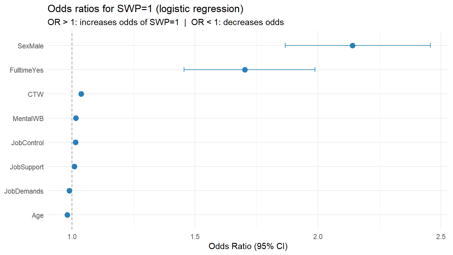
fit <- glm(SWP ~ Age + Sex + Fulltime + CTW + JobDemands + JobControl +
             JobSupport + MentalWB, data = swp, family = binomial)
summary(fit)


Call:
glm(formula = SWP ~ Age + Sex + Fulltime + CTW + JobDemands + 
    JobControl + JobSupport + MentalWB, family = binomial, data = swp)

Coefficients:
             Estimate Std. Error z value Pr(>|z|)    
(Intercept) -4.165661   0.727417  -5.727 1.02e-08 ***
Age         -0.019749   0.002914  -6.778 1.22e-11 ***
SexMale      0.760748   0.069982  10.871  < 2e-16 ***
FulltimeYes  0.532284   0.079393   6.704 2.02e-11 ***
CTW          0.036638   0.003627  10.102  < 2e-16 ***
JobDemands  -0.011014   0.003597  -3.062   0.0022 ** 
JobControl   0.014306   0.003404   4.203 2.63e-05 ***
JobSupport   0.009183   0.003551   2.586   0.0097 ** 
MentalWB     0.015792   0.003518   4.489 7.16e-06 ***
---
Signif. codes:  0 '***' 0.001 '**' 0.01 '*' 0.05 '.' 0.1 ' ' 1

(Dispersion parameter for binomial family taken to be 1)

    Null deviance: 6942.8  on 9999  degrees of freedom
Residual deviance: 6430.4  on 9991  degrees of freedom
AIC: 6448.4

Number of Fisher Scoring iterations: 5

# Odds ratios with 95% CI
or_df <- data.frame(
  variable = names(coef(fit))[-1],
  OR  = exp(coef(fit)[-1]),
  lower = exp(confint(fit)[-1, 1]),
  upper = exp(confint(fit)[-1, 2])
)

Waiting for profiling to be done...
Waiting for profiling to be done...

ggplot(or_df, aes(x = reorder(variable, OR), y = OR)) +
  geom_point(size = 3, colour = "#2980b9") +
  geom_errorbar(aes(ymin = lower, ymax = upper), width = 0.2, colour = "#2980b9") +
  geom_hline(yintercept = 1, linetype = "dashed", colour = "#888") +
  coord_flip() +
  labs(title = "Odds ratios for SWP=1 (logistic regression)",
       subtitle = "OR > 1: increases odds of SWP=1  |  OR < 1: decreases odds",
       x = NULL, y = "Odds Ratio (95% CI)") +
  theme_minimal()

# Default threshold = 0.5
pred_prob <- predict(fit, type = "response")
pred_class <- ifelse(pred_prob > 0.5, 1, 0)

cm <- table(Predicted = pred_class, Actual = swp$SWP)
print(cm)

         Actual
Predicted    0    1
        0   10    5
        1 1093 8892

cat("\nAccuracy:   ", round(mean(pred_class == swp$SWP) * 100, 1), "%\n")


Accuracy:    89 %

cat("Sensitivity:", round(cm[2,2] / sum(cm[,2]) * 100, 1), "% (correctly identified SWP=1)\n")

Sensitivity: 99.9 % (correctly identified SWP=1)

cat("Specificity:", round(cm[1,1] / sum(cm[,1]) * 100, 1), "% (correctly identified SWP=0)\n")

Specificity: 0.9 % (correctly identified SWP=0)

4 Guided Practice

R is loading in the background — exercises below will be interactive once ready.

What to look for

At threshold=0.5, sensitivity for SWP=0 is likely very low — why?
As you lower the threshold, sensitivity for SWP=0 increases but specificity decreases
This trade-off is exactly what the ROC curve (C6) visualises

5 Retrieval Challenge

6 Why-Questions

Q: “Can I use logistic regression with 80 predictors?”

Yes, but with caution. With p=80 and n=10000, OLS-style logistic regression is technically feasible (n >> p), but many of those 80 variables may be redundant questionnaire items. Better to either (a) use penalised logistic regression (LASSO with glmnet, family=“binomial”), or (b) first create composite scores (as was done here with CTW, JobDemands etc.) from the raw items. Blindly including all raw items risks overfitting and obscures interpretation.