In STA220 you used factor analysis (FA) on the HAD scale — 14 items measuring depression and anxiety. FA found two latent factors: one loading on depression items, one on anxiety. Both factors were hidden dimensions that explained the correlations among items.
Both methods reduce many correlated variables to a smaller set of dimensions. PCA is simpler and makes no distributional assumptions — it is purely about variance.
1.2 The geometry of PCA
Given \(n\) observations on \(p\) variables, PCA finds a sequence of orthogonal directions (principal components) \(\mathbf{z}_1, \mathbf{z}_2, \ldots\) such that:
\(\mathbf{V}\): eigenvectors = directions of principal components (loadings)
\(\mathbf{D}\): diagonal matrix of eigenvalues = variance explained by each component
Proportion of variance explained by component \(k\): \(\lambda_k / \sum_j \lambda_j\)
1.3 Reading PCA output
Output
What it tells you
Scree plot
Eigenvalues in decreasing order — look for an “elbow”
Loadings
How much each original variable contributes to each PC
Biplot
Observations (points) and variables (arrows) in PC space
Cumulative variance
How many PCs needed to explain e.g. 80% of variance
1.4 Scaling matters
Always use scale = TRUE in prcomp(). Variables on different scales (age in years, cholesterol in mmol/L) would otherwise be dominated by whichever has the largest variance — purely an artefact of measurement units, not biology.
2 Quiz
PCA would extract more components than FA because it retains all variance, including noise
PCA maximises variance geometrically — no generative model or latent constructs are assumed
PCA and FA give identical factor solutions when fitted to the same data with the same number of factors
PCA requires a labelled response variable Y to guide dimension extraction — FA does not need one
FA assumes X = Λf + ε — latent factors causally produce the observed items. PCA makes no such assumption: it finds orthogonal directions that explain the most variance. On HAD data the first two PCs would likely align with the depression/anxiety split, but a PC is not a "latent factor" — it is a linear combination that maximises explained variance.
2.4% — the raw eigenvalue expressed as a percentage
24% — one fifth of the five eigenvalues
48% — eigenvalue 2.4 divided by the total 5.0 (sum = number of scaled variables)
Indeterminate — eigenvalues alone are insufficient without the raw data
With scale = TRUE, the total variance equals the number of variables (each standardised variable has variance 1). Here total = 2.4 + 1.1 + 0.7 + 0.5 + 0.3 = 5.0. PC1 explains 2.4/5.0 = 48%. The first two PCs together explain (2.4 + 1.1)/5.0 = 70%.
Waist and BMI are completely uncorrelated — they contribute to separate components
Waist and BMI are strongly positively correlated — both load similarly on the same components
Waist causally determines BMI, or the other way around, in this dataset
Both variables are redundant and should be removed from the analysis
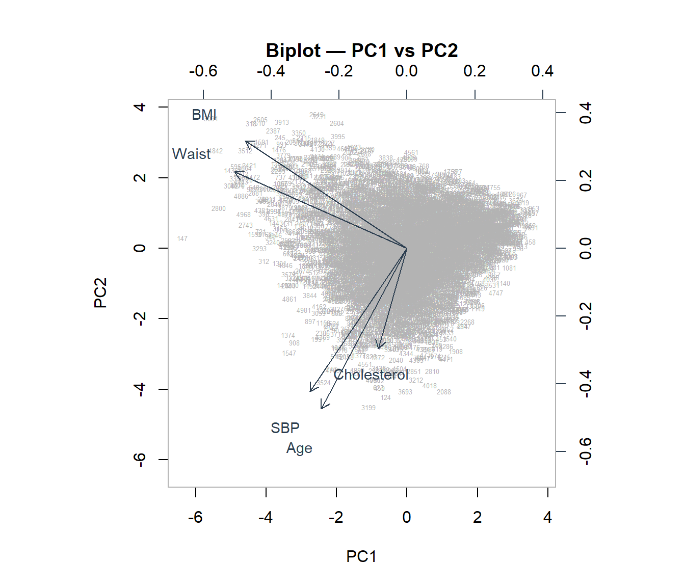
In a biplot, arrows pointing in the same direction indicate variables that move together (are positively correlated). This is exactly what the OLS section identified as multicollinearity between Waist and BMI — PCA reveals this structure visually. One practical use of PCA is to replace correlated predictors with uncorrelated PCs before regression.
3 Worked Example: Health Variables in NHANES
We run PCA on five correlated health variables: Age, BMI, Waist circumference, total Cholesterol, and systolic blood pressure (SBP).
vars <-c("Age", "BMI", "Waist", "Cholesterol", "SBP")X <- nhanes[, vars] |>na.omit() |>scale()pca <-prcomp(X, center =FALSE, scale. =FALSE) # already scaledsummary(pca)
Importance of components:
                          PC1    PC2    PC3    PC4     PC5
Standard deviation     1.4487 1.1570 0.9649 0.7464 0.27300
Proportion of Variance 0.4197 0.2677 0.1862 0.1114 0.01491
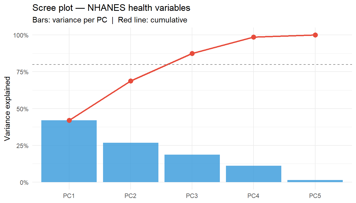
Cumulative Proportion  0.4197 0.6875 0.8737 0.9851 1.00000
var_exp <- pca$sdev^2/sum(pca$sdev^2)cum_var <-cumsum(var_exp)df_scree <-data.frame(PC =factor(paste0("PC", 1:5), levels =paste0("PC", 1:5)),var = var_exp,cum = cum_var)ggplot(df_scree, aes(x = PC, y = var)) +geom_col(fill ="#3498db", alpha =0.8) +geom_line(aes(y = cum, group =1), colour ="#e74c3c", linewidth =1) +geom_point(aes(y = cum), colour ="#e74c3c", size =3) +geom_hline(yintercept =0.8, linetype ="dashed", colour ="grey50") +scale_y_continuous(labels = scales::percent_format()) +labs(title ="Scree plot — NHANES health variables",subtitle ="Bars: variance per PC | Red line: cumulative",x =NULL, y ="Variance explained") +theme_minimal()
Interpretation: PC1 captures the shared “adiposity + cardiovascular burden” axis (BMI, Waist, SBP load positively). PC2 separates Age from the metabolic variables. This mirrors what FA would find, but the components are labelled by variance, not by psychological constructs.
4 Guided Practice
R is loading in the background — the exercises below will be interactive once the status bar disappears.
TipHints
pca$sdev^2 gives eigenvalues; divide by sum(...) for proportions
pca$rotation[, 1] gives loadings on the first PC
Look for the “elbow” in the scree plot — the point where adding more PCs gains little
In the biplot, arrows pointing in the same direction = positively correlated variables
CautionQ: “Can I use PC scores as predictors in regression instead of the original variables?”
Yes — this is called Principal Component Regression (PCR). It solves multicollinearity (BMI + Waist from the OLS page) because PCs are orthogonal by construction. The trade-off: PCs are harder to interpret than original variables, and there is no guarantee that the PCs that explain the most variance in X are the ones most predictive of Y. LASSO and Ridge often outperform PCR because they let the response guide variable selection.
CautionQ: “How is PCA different from what I did in STA220 with Cronbach’s alpha?”
Cronbach’s alpha measures internal consistency — whether items within a scale measure the same construct reliably (high inter-item correlation). PCA finds the direction of maximum variance regardless of reliability. On a well-designed scale like HAD, the first PC will align closely with the sum score (which Cronbach’s alpha validates). But PCA on items with low inter-item correlation still produces components — they just explain less variance and are harder to interpret as constructs.
CautionQ: “Should I use the correlation matrix or the covariance matrix?”
Use the correlation matrix (i.e., scale = TRUE) when variables are on different scales — which is almost always. Using the covariance matrix means variables with larger variances dominate PC1. If you have five health variables measured in different units (years, kg/m², mmol/L, mmHg), the one with the largest raw variance will drive the first component — an artefact of measurement, not biology.
NoteFurther reading
James et al. (2021). An Introduction to Statistical Learning. — Chapter 12.2