R3 — Ridge Regression

1 Concept: Regularisation via L2 Penalty

1.1 The ridge objective

Ridge regression adds an \(L_2\) penalty to the OLS loss:

\[\hat{\boldsymbol{\beta}}^{\text{ridge}} = \arg\min_{\boldsymbol{\beta}} \left\{ \sum_{i=1}^n (y_i - \mathbf{x}_i^\top\boldsymbol{\beta})^2 + \lambda \sum_{j=1}^p \beta_j^2 \right\}\]

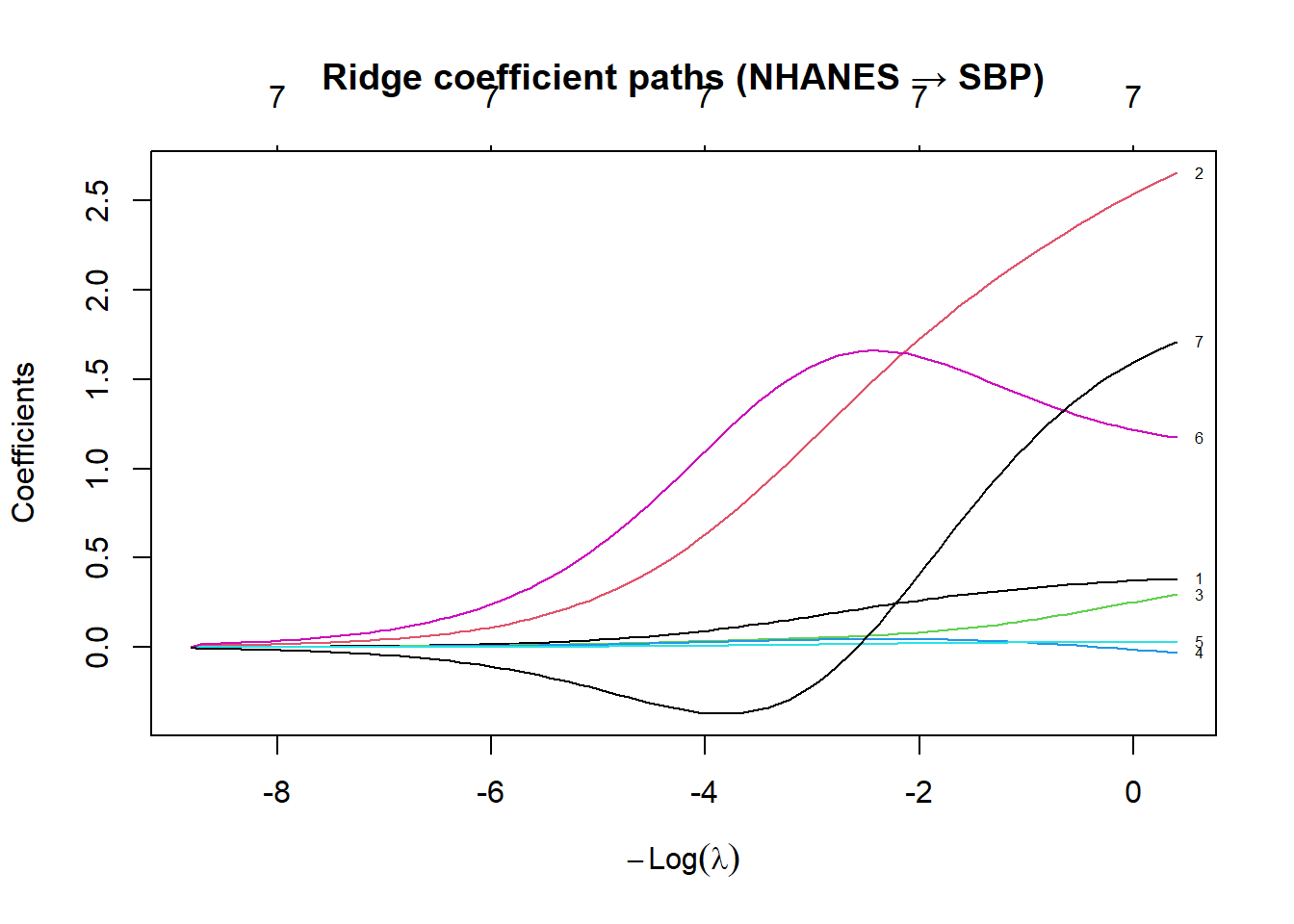
The penalty \(\lambda \sum \beta_j^2\) shrinks all coefficients toward zero. The tuning parameter \(\lambda \geq 0\) controls the amount of shrinkage:

\(\lambda = 0\): OLS (no shrinkage)
\(\lambda \to \infty\): all \(\hat{\beta}_j \to 0\)

1.2 Closed-form solution

\[\hat{\boldsymbol{\beta}}^{\text{ridge}} = (\mathbf{X}^\top\mathbf{X} + \lambda\mathbf{I})^{-1}\mathbf{X}^\top\mathbf{y}\]

Adding \(\lambda\mathbf{I}\) makes the matrix invertible even when \(\mathbf{X}^\top\mathbf{X}\) is singular or near-singular — this is why ridge works when \(p \geq n\).

1.3 Bias-variance effect

\(\lambda\)	Bias	Variance	Test MSE
0 (OLS)	0	High	May be high
Small	Low	Lower	Often lower
Large	High	Very low	May be high

Key insight: Ridge introduces bias but reduces variance. The optimal \(\lambda\) minimises test MSE — found via cross-validation.

1.4 Important: standardise predictors

Ridge shrinks coefficients, but the amount of shrinkage depends on predictor scale. Always standardise predictors before applying ridge (and LASSO). glmnet() does this automatically by default.

2 Quiz

The L2 penalty is simply not large enough mathematically to force any coefficient to exactly zero

The L2 gradient 2λβ → 0 as β → 0, so the optimal β is always small but never exactly zero

A smooth L2 penalty has no kink at zero, unlike L1, so it cannot produce exact sparse solutions

Ridge zeros out large coefficients while leaving small coefficients unchanged by the L2 penalty

The L2 penalty contributes a gradient of 2λβ_j to each coefficient. As β_j gets small, the gradient also gets small — so the optimum is at some small but non-zero value. In contrast, the L1 penalty (LASSO) has a constant subgradient of λ near zero, which forces the optimum to exactly zero for small enough coefficients. This is why LASSO performs variable selection and ridge does not.

Only a few predictors truly affect the outcome

Many predictors each have a small true effect

Predictors are independent of each other

You need an interpretable sparse solution

Ridge is best when the true signal is spread across many predictors — it shrinks all coefficients moderately. LASSO is best when only a few predictors truly matter — it zeros out the rest. In GWAS (genetic association studies), for example, many thousands of SNPs each have tiny effects — ridge is often preferred. For clinical risk scores, LASSO is preferred for sparsity.

Ridge breaks down entirely when predictors have different scales — the algorithm cannot produce a solution

Large-scale predictors have bigger β² and face more penalty shrinkage than small-scale ones

The algorithm fails to converge numerically when predictors span very different measurement scales

No problem — the ridge penalty automatically adjusts for predictor scale before applying shrinkage

The L2 penalty is λΣβ_j². A predictor measured in large units (like Cholesterol in mg/dL) will have a small coefficient even for a strong association — so its coefficient gets penalised less. A predictor in small units has a large coefficient even for a weak effect — and gets penalised more. Standardising removes this scale dependence. glmnet() standardises by default.

3 Worked Example

set.seed(42)
# glmnet with alpha=0 is ridge
# By default standardises predictors and fits over a lambda grid
ridge_fit <- glmnet(X, y, alpha = 0)

# Coefficient paths
plot(ridge_fit, xvar = "lambda", label = TRUE,
     main = "Ridge coefficient paths (NHANES → SBP)")

# 10-fold CV to find optimal lambda
set.seed(42)
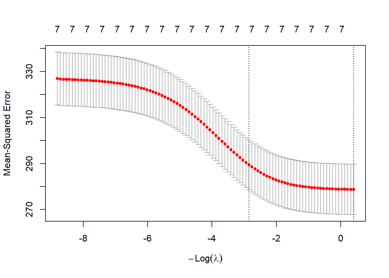
cv_ridge <- cv.glmnet(X, y, alpha = 0, nfolds = 10)
plot(cv_ridge)

cat("lambda.min:", round(cv_ridge$lambda.min, 4), "\n")

lambda.min: 0.6682

cat("lambda.1se:", round(cv_ridge$lambda.1se, 4), "\n")

lambda.1se: 17.3403

cat("\nCV RMSPE at lambda.min:", round(sqrt(min(cv_ridge$cvm)), 3), "mmHg\n")


CV RMSPE at lambda.min: 16.695 mmHg

# Compare ridge vs OLS on a train/test split
set.seed(42)
tr_idx <- sample(nrow(nhanes_cc), round(0.7 * nrow(nhanes_cc)))
X_tr <- X[tr_idx, ];   y_tr <- y[tr_idx]
X_te <- X[-tr_idx, ];  y_te <- y[-tr_idx]

ols_fit   <- lm(y_tr ~ X_tr)
ridge_cv  <- cv.glmnet(X_tr, y_tr, alpha = 0, nfolds = 10)

ols_rmspe   <- sqrt(mean((y_te - cbind(1, X_te) %*% coef(ols_fit))^2))
ridge_rmspe <- sqrt(mean((y_te - predict(ridge_cv, newx = X_te, s = "lambda.min"))^2))

cat("OLS test RMSPE:   ", round(ols_rmspe,   3), "mmHg\n")

OLS test RMSPE:    17.368 mmHg

cat("Ridge test RMSPE: ", round(ridge_rmspe, 3), "mmHg\n")

Ridge test RMSPE:  17.398 mmHg

4 Guided Practice

R is loading in the background — exercises below will be interactive once ready.

What to compare

Are the ridge coefficients larger or smaller than OLS?
Which predictor is shrunk the most? Does that make sense?
Does the ridge RMSPE meaningfully beat OLS here? (With n=4000+ and p=7, shrinkage may help little)

5 Why-Questions

Q: “Ridge keeps all predictors. How is that useful for interpretation?”

Ridge is primarily a prediction method, not an inference method. If interpretation matters, report OLS coefficients (with SE and p-values) from a carefully selected model. Use ridge when your goal is accurate prediction with many correlated predictors — for example, predicting future SBP from a panel of biomarkers. The stability of ridge coefficients under collinearity is a feature, not a bug, for prediction purposes.

Q: “Does it matter if I standardise before or inside glmnet?”

glmnet() standardises internally by default (standardize=TRUE), fits on the standardised scale, then returns coefficients on the original scale. This means you can pass raw data and interpret coefficients directly. If you standardise manually first, set standardize=FALSE. Never standardise the outcome y for ridge/LASSO regression — only the predictors X.