C6 — ROC Curve & AUC

1 Concept: Evaluating Classifiers Beyond Accuracy

1.1 The confusion matrix

For binary classification with threshold \(c\): classify as positive if \(\hat{p} > c\).

	Actual +	Actual −
Predicted +	TP	FP
Predicted −	FN	TN

Key metrics:

\[\text{Sensitivity} = \frac{TP}{TP + FN} \quad \text{(true positive rate, recall)}\] \[\text{Specificity} = \frac{TN}{TN + FP} \quad \text{(true negative rate)}\] \[\text{PPV (Precision)} = \frac{TP}{TP + FP}\]

1.2 The ROC curve

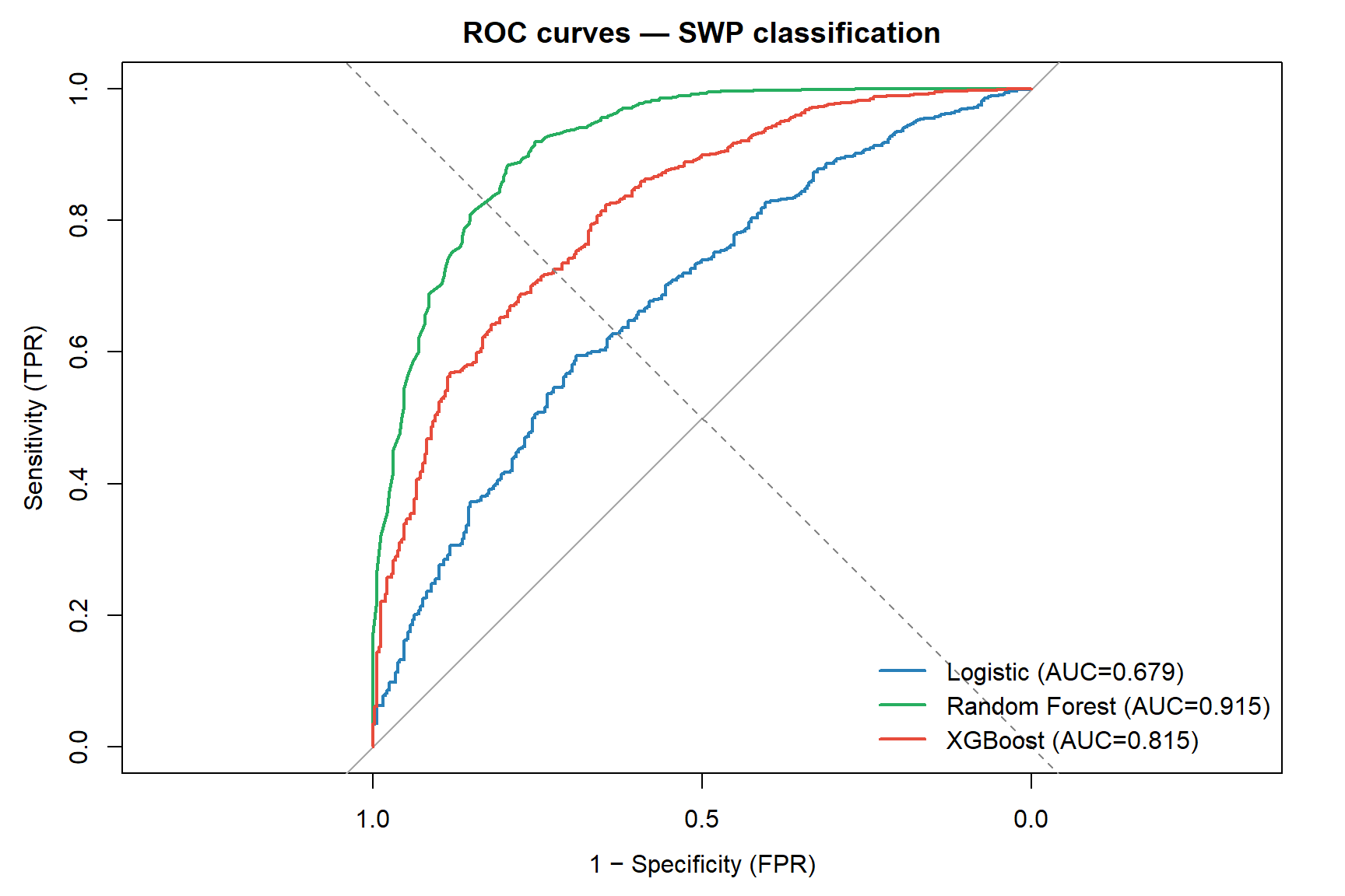
The Receiver Operating Characteristic curve plots sensitivity (TPR) vs 1−specificity (FPR) as the threshold \(c\) varies from 0 to 1.

Top-left corner (TPR=1, FPR=0): perfect classifier
Diagonal (TPR = FPR): random classifier
AUC (Area Under the Curve): probability that a randomly chosen positive example scores higher than a randomly chosen negative example — ranges 0.5 (random) to 1.0 (perfect)

1.3 Choosing a threshold

The optimal threshold depends on the cost asymmetry:

In occupational health: missing a worker at risk (FN) may be more costly than a false alarm (FP) → lower threshold → higher sensitivity
Rule: choose threshold that maximises \(\text{Sensitivity} + \text{Specificity} - 1\) (Youden’s J) or matches clinical cost-benefit

1.4 Discrimination vs calibration

These are two distinct, independent model properties:

Aspect	Question	Metrics
Discrimination	Can the model rank positives above negatives?	AUC / C-statistic, sensitivity, specificity
Calibration	Are the predicted probabilities accurate?	Calibration plot, Hosmer-Lemeshow, Brier score

A model can discriminate well but be poorly calibrated — e.g., it ranks workers correctly but systematically overestimates risk. For clinical and public health decision-making, both must be reported.

1.5 Calibration metrics

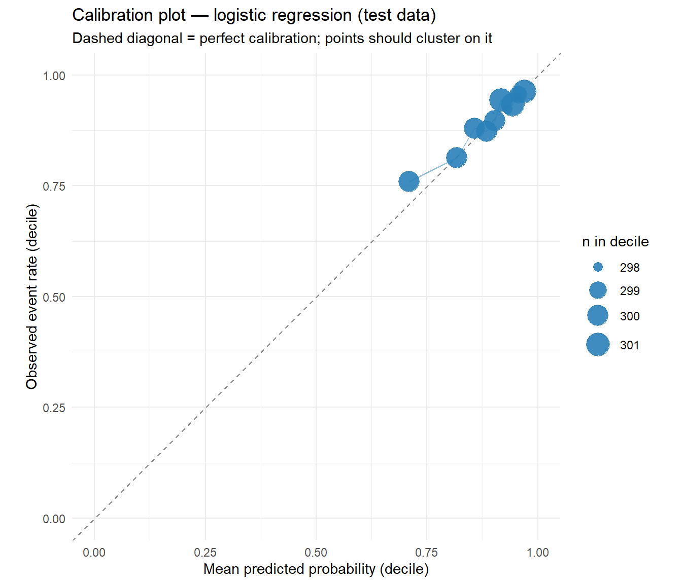
Calibration plot: Group predicted probabilities into deciles. Compare the mean predicted probability to the observed event rate in each group. Points on the diagonal = perfect calibration.

Hosmer-Lemeshow test: Chi-squared test for calibration across \(g\) groups (usually 10). Non-significant \(p\) value = no evidence of poor calibration. Note: the test has low power in small samples.

Brier score: Mean squared error of predicted probabilities.

\[\text{BS} = \frac{1}{n}\sum_{i=1}^{n}(\hat{p}_i - y_i)^2\]

Ranges 0 (perfect) to 1. For a balanced outcome, a random (0.5 always) classifier gives BS = 0.25.

1.6 Kappa statistic

Cohen’s kappa corrects accuracy for chance agreement:

\[\kappa = \frac{p_o - p_e}{1 - p_e}\]

where \(p_o\) is observed accuracy and \(p_e\) is accuracy expected by chance (based on marginal distributions). Interpretation: \(\kappa = 0\) means no better than chance; \(\kappa > 0.6\) is substantial agreement; \(\kappa > 0.8\) is almost perfect.

Imbalanced data and misleading accuracy

With 89% SWP=1 in the SWP dataset, always predicting SWP=1 achieves 89% accuracy — but \(\kappa = 0\). Accuracy is misleading when classes are imbalanced. Report AUC and sensitivity alongside accuracy, and always check kappa.

2 Quiz

The model correctly classifies 75% of all observations at the 0.5 threshold

For a random positive-negative pair, the model ranks the positive higher 75% of the time

The model achieves exactly 75% sensitivity and 75% specificity simultaneously

75% of the area under the precision-recall curve is captured by the model

AUC is a rank-based metric: it measures how well the model separates the two classes in terms of predicted probability. AUC=0.5 means random ordering (no discrimination). AUC=1.0 means all positives score higher than all negatives. AUC=0.75 means 75% of positive-negative pairs are correctly ranked. Crucially, AUC is threshold-independent — it evaluates the model's discrimination ability regardless of where you place the cutoff.

Model A — higher accuracy is always the primary criterion

Model B — better AUC means better discrimination; model A's accuracy likely reflects majority-class prediction

They are equivalent — accuracy and AUC always agree

Model A — AUC is only valid for balanced datasets

With 89% majority class (SWP=1), model A's 92% accuracy likely comes from correctly predicting SWP=1 for almost everyone. AUC=0.61 is barely above random — it has almost no ability to rank the minority class (SWP=0) above the majority. Model B sacrifices 3% accuracy but dramatically improves discrimination. For identifying at-risk workers, AUC (or sensitivity at a clinically chosen threshold) is the right metric.

Increase the threshold above 0.5

Lower the threshold below 0.5 — classifying more as positive increases sensitivity at the cost of specificity

Keep the threshold at 0.5 — that is always optimal

Use AUC instead of a threshold — it avoids threshold choice entirely

Lowering the threshold means more observations are classified as positive (SWP=0 risk, requiring intervention). This increases sensitivity (fewer at-risk workers missed) but decreases specificity (more false alarms — workers who would have been fine are flagged). The optimal threshold depends on the relative costs of FN vs FP in the specific application. The ROC curve shows you all possible (FPR, TPR) trade-offs simultaneously.

The model has poor discrimination — it cannot rank positives above negatives

Good discrimination but poor calibration — the predicted probabilities do not match actual event rates

The AUC estimate is statistically unreliable

The model has overfit the training data

Discrimination and calibration are independent. AUC = 0.83 means the model ranks 83% of positive–negative pairs correctly — good discrimination. Hosmer-Lemeshow p = 0.01 means the predicted probabilities are systematically off in some probability range — poor calibration. You can have excellent discrimination with poor calibration (e.g., all predicted probabilities shifted upward by 0.2). For clinical use you need both: accurate ranking AND accurate probability estimates.

0.89 — the model correctly classifies 89% of observations

≈ 0 — after correcting for the class imbalance, the model performs no better than chance

Negative — the model is worse than random

Cannot be calculated without a confusion matrix

κ = (p_o − p_e) / (1 − p_e). p_o = 0.89 (accuracy). p_e = expected accuracy by chance = (probability predict 1)(probability actual 1) + (prob. predict 0)(prob. actual 0) = 1.0 × 0.89 + 0.0 × 0.11 = 0.89. κ = (0.89 − 0.89)/(1 − 0.89) = 0. The model learns nothing beyond the base rate. Kappa exposes what accuracy hides with imbalanced outcomes.

3 Worked Example: ROC Comparison Across All Methods

library(pROC)

# Logistic regression
logit <- glm(SWP ~ Age + Sex + Fulltime + CTW + JobDemands +
               JobControl + JobSupport + MentalWB, data=train, family=binomial)
p_logit <- predict(logit, newdata=test, type="response")

# Random forest
rf <- randomForest(factor(SWP) ~ Age + Sex + Fulltime + CTW + JobDemands +
                     JobControl + JobSupport + MentalWB,
                   data=train_f, ntree=300)
p_rf <- predict(rf, newdata=test_f, type="prob")[, "1"]

# XGBoost
xgb_fit <- xgb.train(
  params  = list(objective="binary:logistic", eta=0.1, max_depth=4,
                 eval_metric="auc"),
  data    = dtrain, nrounds=200, verbose=0)
p_xgb <- predict(xgb_fit, dtest)

# ROC curves
roc_logit <- roc(test$SWP, p_logit, quiet=TRUE)
roc_rf    <- roc(test$SWP, p_rf,    quiet=TRUE)
roc_xgb   <- roc(test$SWP, p_xgb,  quiet=TRUE)

# Plot
plot(roc_logit, col="#2980b9", lwd=2,
     main="ROC curves — SWP classification",
     xlab="1 − Specificity (FPR)", ylab="Sensitivity (TPR)")
lines(roc_rf,  col="#27ae60", lwd=2)
lines(roc_xgb, col="#e74c3c", lwd=2)
abline(0, 1, lty=2, col="#888")
legend("bottomright",
       legend=c(paste0("Logistic (AUC=", round(auc(roc_logit),3), ")"),
                paste0("Random Forest (AUC=", round(auc(roc_rf),3), ")"),
                paste0("XGBoost (AUC=", round(auc(roc_xgb),3), ")")),
       col=c("#2980b9","#27ae60","#e74c3c"), lwd=2, bty="n")

# Find optimal threshold for logistic model (Youden's J)
coords_logit <- coords(roc_logit, "best", best.method="youden")
cat("Optimal threshold (Youden):", round(coords_logit$threshold, 4), "\n")

Optimal threshold (Youden): 0.9009

cat("  Sensitivity:", round(coords_logit$sensitivity*100, 1), "%\n")

  Sensitivity: 59.5 %

cat("  Specificity:", round(coords_logit$specificity*100, 1), "%\n")

  Specificity: 69.1 %

# Compare to default threshold=0.5
pred_05  <- ifelse(p_logit > 0.5, 1, 0)
pred_opt <- ifelse(p_logit > coords_logit$threshold, 1, 0)

cm_05  <- table(Predicted=pred_05,  Actual=test$SWP)
cm_opt <- table(Predicted=pred_opt, Actual=test$SWP)

cat("\nThreshold=0.5:\n")


Threshold=0.5:

cat("  Sensitivity (SWP=0):", round(cm_05[1,1]/sum(cm_05[,1])*100,1), "%\n")

  Sensitivity (SWP=0): 2.2 %

cat("  Accuracy:           ", round(mean(pred_05==test$SWP)*100,1), "%\n")

  Accuracy:            89.6 %

cat("\nThreshold=", round(coords_logit$threshold,3), "(Youden):\n")


Threshold= 0.901 (Youden):

cat("  Sensitivity (SWP=0):", round(cm_opt[1,1]/sum(cm_opt[,1])*100,1), "%\n")

  Sensitivity (SWP=0): 69.1 %

cat("  Accuracy:           ", round(mean(pred_opt==test$SWP)*100,1), "%\n")

  Accuracy:            60.5 %

3.1 Calibration: are the predicted probabilities accurate?

# Decile-based calibration plot for logistic regression
cal_df <- data.frame(pred = p_logit, obs = test$SWP)
cal_df$decile <- as.integer(cut(rank(cal_df$pred), breaks = 10, labels = FALSE))
cal_sum <- cal_df |>
  dplyr::group_by(decile) |>
  dplyr::summarise(mean_pred = mean(pred),
                   mean_obs  = mean(obs),
                   n         = dplyr::n(),
                   .groups   = "drop")

ggplot(cal_sum, aes(mean_pred, mean_obs)) +
  geom_abline(slope = 1, intercept = 0, linetype = "dashed", colour = "#888") +
  geom_line(colour = "#2980b9", alpha = 0.5) +
  geom_point(aes(size = n), colour = "#2980b9", alpha = 0.9) +
  scale_size_continuous(range = c(3, 8), name = "n in decile") +
  coord_equal(xlim = c(0, 1), ylim = c(0, 1)) +
  labs(title = "Calibration plot — logistic regression (test data)",
       subtitle = "Dashed diagonal = perfect calibration; points should cluster on it",
       x = "Mean predicted probability (decile)",
       y = "Observed event rate (decile)") +
  theme_minimal()

# Brier score — mean squared error of predicted probabilities
brier <- mean((p_logit - test$SWP)^2)

# Kappa — corrects accuracy for chance agreement
pred_05 <- ifelse(p_logit > 0.5, 1, 0)
po <- mean(pred_05 == test$SWP)
pe <- mean(pred_05 == 0) * mean(test$SWP == 0) +
      mean(pred_05 == 1) * mean(test$SWP == 1)
kappa_val <- (po - pe) / (1 - pe)

cat("=== Model evaluation summary (logistic, test data) ===\n")

=== Model evaluation summary (logistic, test data) ===

cat(sprintf("\nDiscrimination:\n"))


Discrimination:

cat(sprintf("  AUC (C-statistic):    %.3f\n", as.numeric(auc(roc_logit))))

  AUC (C-statistic):    0.679

cat(sprintf("\nCalibration:\n"))


Calibration:

cat(sprintf("  Brier score:          %.4f  (lower = better; 0 = perfect)\n", brier))

  Brier score:          0.0904  (lower = better; 0 = perfect)

cat(sprintf("\nClassification (threshold = 0.5):\n"))


Classification (threshold = 0.5):

cat(sprintf("  Accuracy:             %.1f%%\n", po * 100))

  Accuracy:             89.6%

cat(sprintf("  Kappa:                %.4f  (0 = chance, >0.6 = substantial)\n", kappa_val))

  Kappa:                0.0366  (0 = chance, >0.6 = substantial)

cat(sprintf("  Sensitivity (SWP=0):  %.1f%%\n",
    round(cm_05[1,1] / sum(cm_05[,1]) * 100, 1)))

  Sensitivity (SWP=0):  2.2%

4 Guided Practice

R is loading in the background — exercises below will be interactive once ready.

Clinical interpretation

In occupational health, a worker flagged as SWP=0 (at risk) would receive an intervention. The costs are: - False negative (missed): worker deteriorates without support — high cost - False positive (false alarm): unnecessary intervention — lower cost

This asymmetry justifies a low threshold (favour sensitivity) and reporting sensitivity alongside AUC rather than accuracy.

5 Why-Questions

Q: “AUC of 0.80 — is that good?”

It depends on the application. General benchmarks: - 0.5: random (no discrimination) - 0.7–0.8: acceptable - 0.8–0.9: excellent - > 0.9: outstanding (sometimes suspicious — check for data leakage)

For predicting sustainable work participation from self-reported scales (which have measurement error), AUC ≈ 0.75–0.85 is realistic and clinically useful. Higher AUC in this setting might indicate overfitting or a leaking predictor.

Q: “Should I report AUC or the precision-recall curve?”

For imbalanced datasets, the precision-recall (PR) curve is often more informative than ROC: - ROC AUC can look high even when sensitivity for the minority class is poor - PR curve focuses on the minority class performance - pROC::plot.roc() shows ROC; use PRROC package for PR curves

In clinical settings, always report both — and report sensitivity and specificity at the chosen operating threshold.