C2 — LDA & kNN

1 Concept: Generative Classifiers and Distance Methods

1.1 Linear Discriminant Analysis (LDA)

LDA models the class-conditional distributions \(P(\mathbf{X} \mid Y=k)\) as multivariate Gaussians with the same covariance matrix \(\boldsymbol{\Sigma}\). Via Bayes’ theorem, this gives a linear decision boundary. QDA relaxes equal-covariance, giving a quadratic boundary but estimating more parameters.

1.2 k-Nearest Neighbours (kNN)

kNN is non-parametric — no distributional assumption:

For a new point \(\mathbf{x}_0\), find the \(k\) closest training points
Assign the majority class among those neighbours

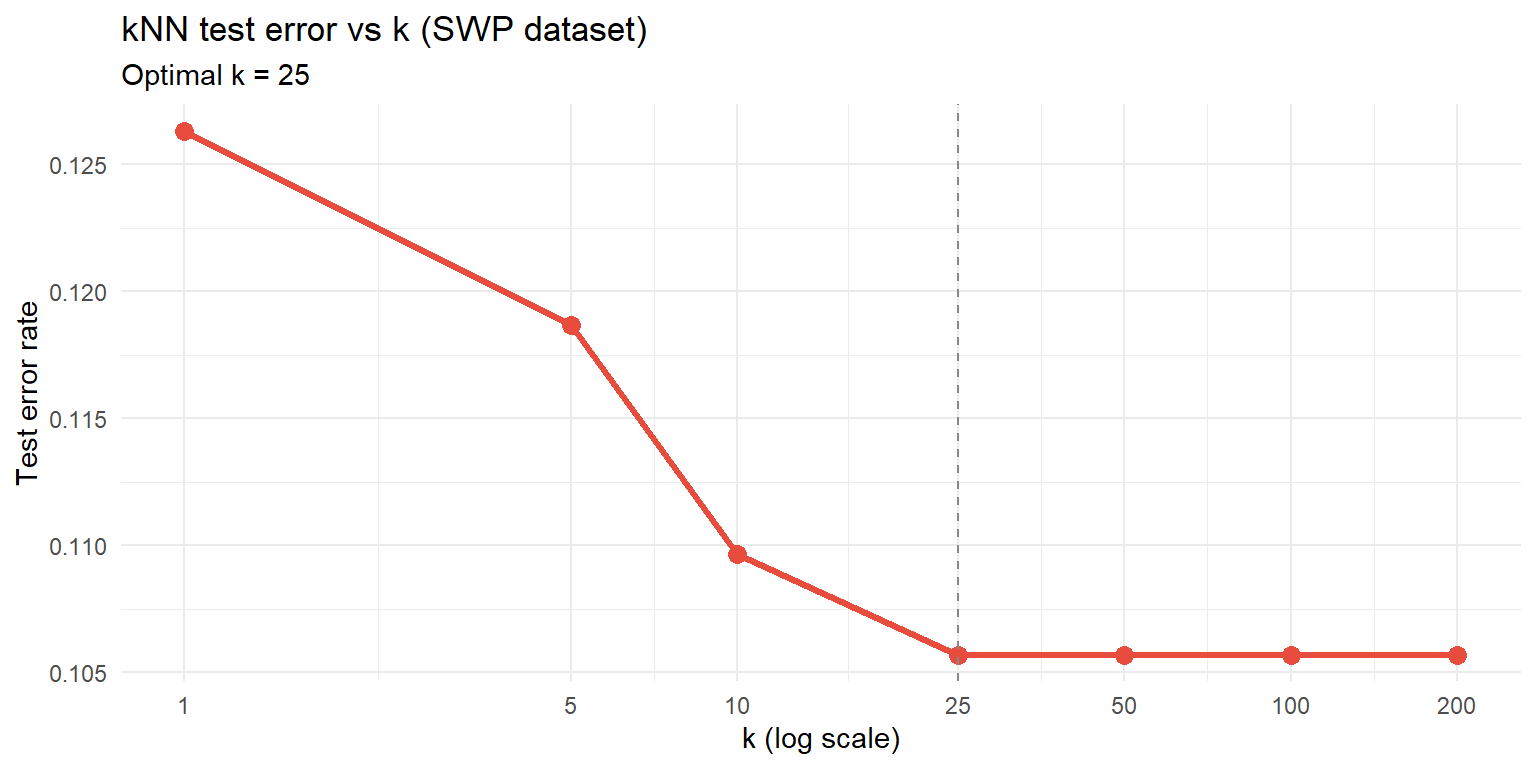
Small \(k\) = flexible, low bias, high variance. Large \(k\) = smooth, high bias, low variance. Optimal \(k\) found by cross-validation.

Method	Boundary	Assumption	Scale-sensitive?
Logistic	Linear	None	No
LDA	Linear	Gaussian, equal Σ	No
QDA	Quadratic	Gaussian, different Σ	No
kNN	Non-linear	None	Yes — must standardise

2 Quiz

LDA becomes equivalent to logistic regression

LDA fails completely and cannot produce predictions

The linear boundary is misspecified — QDA or a flexible method may perform better

LDA automatically corrects by estimating separate covariance matrices

If classes have different covariance structures, the true Bayes boundary is quadratic, not linear. LDA's linear boundary will then be suboptimal. QDA estimates a separate Σ_k per class, giving a quadratic boundary. However, QDA has more parameters and needs more data. With limited data, LDA's lower variance may still outweigh the bias from the wrong boundary shape.

Zero — each training point is its own nearest neighbour

Equal to the Bayes error rate

Equal to 1/n

Undefined — kNN cannot be evaluated on training data

With k=1, every training point is its own nearest neighbour and is classified perfectly — training error is 0. This is extreme overfitting. Test error with k=1 is much higher. As k increases, the model smooths out and test error first falls then rises — the same U-shape as the bias-variance tradeoff.

kNN requires all predictors to follow a normal distribution so that Euclidean distance is valid

High-range predictors dominate Euclidean distance regardless of their actual predictive importance

Standardisation only speeds up computation — the same neighbours are found regardless of scale

kNN requires integer-valued predictors because Euclidean distance is undefined for continuous inputs

kNN uses Euclidean distance. If Age ranges 18–70 and JobControl ranges 85–120, a 1-unit difference in Age contributes more to distance than a 1-unit difference in JobControl — even if JobControl is more informative. Standardising (subtract mean, divide by SD) puts all predictors on equal footing and is essential before kNN.

3 Worked Example

lda_fit  <- lda(SWP ~ Age + CTW + JobDemands + JobControl + JobSupport + MentalWB,
                data = train)
lda_pred <- predict(lda_fit, newdata = test)
cm_lda   <- table(Predicted = lda_pred$class, Actual = test$SWP)
print(cm_lda)

         Actual
Predicted    0    1
        0    1    1
        1  316 2682

cat("\nTest accuracy:      ", round(mean(lda_pred$class == test$SWP)*100, 1), "%\n")


Test accuracy:       89.4 %

cat("Sensitivity (SWP=0):", round(cm_lda[1,1] / sum(cm_lda[,1])*100, 1), "%\n")

Sensitivity (SWP=0): 0.3 %

cat("Specificity (SWP=1):", round(cm_lda[2,2] / sum(cm_lda[,2])*100, 1), "%\n")

Specificity (SWP=1): 100 %

pred_vars <- c("Age","CTW","JobDemands","JobControl","JobSupport","MentalWB")
mu  <- colMeans(train[, pred_vars])
sds <- apply(train[, pred_vars], 2, sd)
X_tr <- scale(train[, pred_vars], center = mu, scale = sds)
X_te <- scale(test[, pred_vars],  center = mu, scale = sds)

# Use a subset for speed during rendering (n=7000 kNN is slow)
set.seed(7)
sub <- sample(nrow(X_tr), 1500)
X_tr_s <- X_tr[sub, ]; y_tr_s <- train$SWP[sub]

ks        <- c(1, 5, 10, 25, 50, 100, 200)
test_err  <- sapply(ks, function(k) mean(knn(X_tr_s, X_te, cl = y_tr_s, k=k) != test$SWP))

ggplot(data.frame(k = ks, error = test_err), aes(k, error)) +
  geom_line(colour="#e74c3c", linewidth=1.2) +
  geom_point(size=3, colour="#e74c3c") +
  geom_vline(xintercept=ks[which.min(test_err)], linetype="dashed", colour="#888") +
  scale_x_log10(breaks=ks) +
  labs(title="kNN test error vs k (SWP dataset)",
       subtitle=paste0("Optimal k = ", ks[which.min(test_err)]),
       x="k (log scale)", y="Test error rate") +
  theme_minimal()

logit    <- glm(SWP ~ Age + CTW + JobDemands + JobControl + JobSupport + MentalWB,
                data=train, family=binomial)
k_best   <- ks[which.min(test_err)]
knn_pred <- knn(X_tr_s, X_te, cl=y_tr_s, k=k_best)

cat("Test accuracy:\n")

Test accuracy:

cat("  Null (always SWP=1):    ", round(mean(test$SWP==1)*100,1), "%\n")

  Null (always SWP=1):     89.4 %

cat("  Logistic regression:    ", round(mean(ifelse(predict(logit,test,type="response")>0.5,1,0)==test$SWP)*100,1), "%\n")

  Logistic regression:     89.4 %

cat("  LDA:                    ", round(mean(lda_pred$class==test$SWP)*100,1), "%\n")

  LDA:                     89.4 %

cat("  kNN (k=", k_best, "):          ", round(mean(knn_pred==test$SWP)*100,1), "%\n")

  kNN (k= 25 ):           89.4 %

4 Guided Practice

R is loading in the background — exercises below will be interactive once ready.