C4 — Random Forests

1 Concept: Ensemble Learning via Bagging and Random Forests

1.1 Bagging: reducing variance by averaging

A single tree has high variance. Bagging (Bootstrap Aggregating) reduces variance by averaging many trees:

Draw \(B\) bootstrap samples (size \(n\) with replacement) from training data
Fit a full tree on each bootstrap sample
Predict by majority vote across all \(B\) trees

Since each tree is trained on a different sample, averaging \(B\) uncorrelated trees reduces variance by factor \(B\) — while keeping bias approximately constant.

1.2 Random forests: decorrelating trees

In bagging, if one predictor is very strong, most trees will use it at the top split — the trees are correlated. Averaging correlated trees reduces variance less effectively.

Random forests fix this by randomly selecting \(m\) predictors at each split (default: \(m = \sqrt{p}\) for classification). This decorrelates the trees and further reduces variance.

1.3 Key hyperparameters

Parameter	Default	Effect
`ntree`	500	More trees → more stable; diminishing returns
`mtry`	√p	Smaller → more decorrelated, higher bias
`nodesize`	1	Larger → shallower trees, less overfit

1.4 Out-of-bag (OOB) error

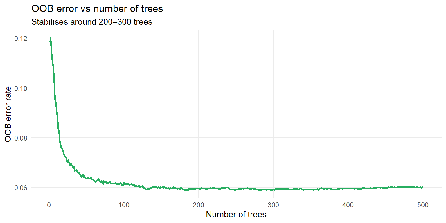
Each tree is trained on ~63% of data (the bootstrap sample). The remaining ~37% (out-of-bag) can be used to estimate test error without a separate validation set. OOB error is a nearly unbiased estimate of test error.

1.5 Variable importance and SHAP values

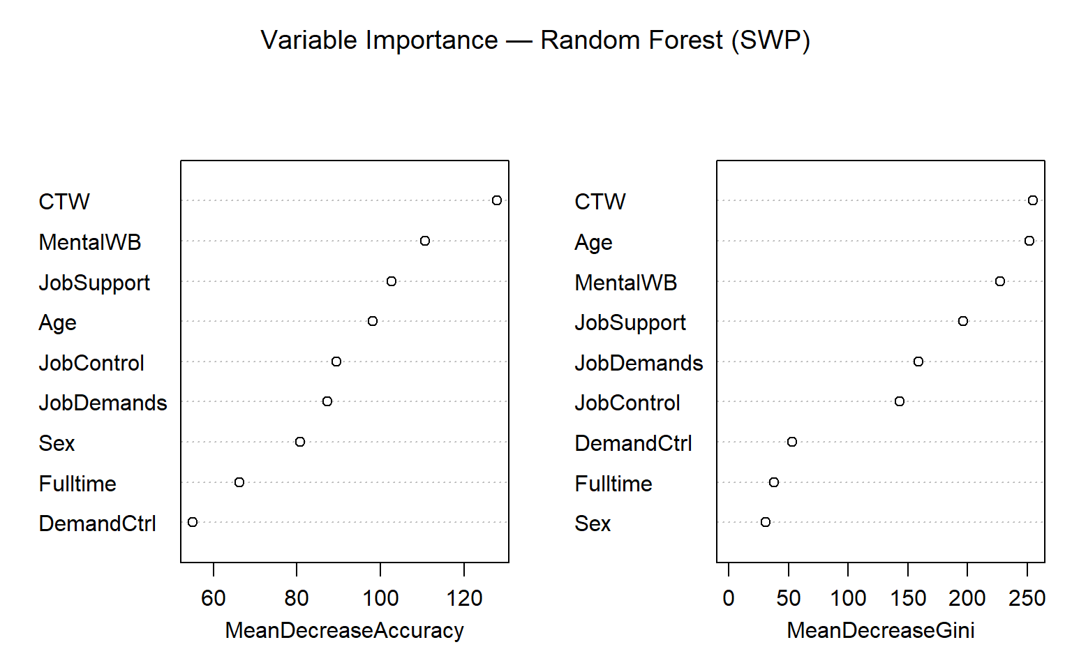
Variable importance in random forests = average decrease in Gini impurity from all splits on a variable, averaged across all trees. A high value means the variable is both frequently used and creates pure splits.

However, importance scores tell you which variables matter but not how they contribute for an individual observation. SHAP (SHapley Additive exPlanations) solves this.

1.5.1 The Shapley intuition

Imagine you want to attribute a predicted value to each predictor. For a model with age = 60 and BMI = 30 (and a bias of 50):

Predictors used	Prediction
{none}	50
{age=60}	70
{BMI=30}	85
{age=60, BMI=30}	100

The Shapley value for age averages its marginal contribution across all orderings:

Adding age first: \(70 - 50 = 20\)
Adding age after BMI: \(100 - 85 = 15\)
SHAP(age) \(= (20 + 15)/2 = 17.5\)

Unlike standardised regression coefficients (which are constant for every individual), SHAP values can differ for each observation — reflecting non-linear and interaction effects that trees capture naturally.

SHAP vs linear regression

In a linear model, the contribution of BMI is always \(\hat{\beta}_{\text{BMI}} \times \text{BMI}_i\) — a constant slope. With a random forest, SHAP might show a steep increase in contribution for very low BMI but a flat contribution in the normal range. This is the key advantage of tree-based SHAP over regression coefficients.

2 Quiz

It reduces computation by evaluating only m < p predictors at each node

Tree decorrelation — without it all trees use the same top predictor and become highly correlated

It introduces randomness that beneficially increases the variance of each individual tree

It prevents overfitting by hard-limiting the maximum depth of each individual tree

If one predictor is dominant (e.g., CTW strongly predicts SWP), all bagged trees will use it at the first split — making the trees highly correlated. Averaging correlated variables reduces variance by σ²/B + (1−1/B)·ρ·σ² — the ρ term prevents full variance reduction. Random forests reduce ρ by hiding the dominant predictor from some splits, making trees more independent and variance reduction more effective.

The average training error across all trees in the ensemble

An honest test-error estimate — each observation is scored only by trees trained without it

The bias of the ensemble, measuring how far predictions are from the truth

The error on 12% of the training data that was deliberately held out

In each bootstrap sample, about 37% of observations are not included (out-of-bag). For each observation, we can predict it using only the trees trained without it — giving an honest test-like estimate. The average OOB error across all observations closely approximates the leave-one-out CV error and doesn't require a separate validation set.

The variable has a large coefficient in a linear model fitted to the forest predictions

This variable's splits consistently create purer child nodes and is frequently used across many trees

The variable is used in every tree's first split

The variable has low correlation with the outcome

Variable importance = total decrease in Gini impurity from all splits on that variable, averaged over all trees. High importance means the variable is both frequently split on (it is useful) and creates pure splits (the classes are well-separated). Unlike a single tree's top split, this averages over many trees and is more stable. Note: it measures predictive importance, not causal importance.

3 Worked Example

library(randomForest)
set.seed(42)
rf_fit <- randomForest(SWP ~ Age + Sex + Fulltime + CTW + JobDemands +
                         JobControl + JobSupport + MentalWB + DemandCtrl,
                       data = train, ntree = 500,
                       importance = TRUE)
print(rf_fit)


Call:
 randomForest(formula = SWP ~ Age + Sex + Fulltime + CTW + JobDemands +      JobControl + JobSupport + MentalWB + DemandCtrl, data = train,      ntree = 500, importance = TRUE) 
               Type of random forest: classification
                     Number of trees: 500
No. of variables tried at each split: 3

        OOB estimate of  error rate: 6.01%
Confusion matrix:
    0    1 class.error
0 401  385  0.48982188
1  36 6178  0.00579337

varImpPlot(rf_fit, main = "Variable Importance — Random Forest (SWP)")

pred_rf <- predict(rf_fit, newdata = test)
cm_rf   <- table(Predicted = pred_rf, Actual = test$SWP)
print(cm_rf)

         Actual
Predicted    0    1
        0  164   11
        1  153 2672

cat("\nTest accuracy:      ", round(mean(pred_rf == test$SWP)*100, 1), "%\n")


Test accuracy:       94.5 %

cat("Sensitivity (SWP=0):", round(cm_rf[1,1]/sum(cm_rf[,1])*100, 1), "%\n")

Sensitivity (SWP=0): 51.7 %

cat("Specificity (SWP=1):", round(cm_rf[2,2]/sum(cm_rf[,2])*100, 1), "%\n")

Specificity (SWP=1): 99.6 %

cat("OOB error:          ", round(rf_fit$err.rate[500,"OOB"]*100, 1), "%\n")

OOB error:           6 %

# OOB error vs number of trees
oob_df <- data.frame(ntree = 1:500, oob = rf_fit$err.rate[,"OOB"])
ggplot(oob_df, aes(ntree, oob)) +
  geom_line(colour="#27ae60", linewidth=1) +
  labs(title="OOB error vs number of trees",
       subtitle="Stabilises around 200–300 trees",
       x="Number of trees", y="OOB error rate") +
  theme_minimal()

4 Guided Practice

R is loading in the background — exercises below will be interactive once ready.

What to look for

Does the random forest improve sensitivity for SWP=0 compared to a single tree (C3)?
Which variable has the highest importance? Does it match the first split of the CART tree?
How does mtry affect the trade-off between accuracy and sensitivity?

5 Why-Questions

Q: “Random forests are hard to interpret. Can I still get insights from them?”

Yes — through variable importance plots and partial dependence plots: - Variable importance: which predictors matter most (but not how or in which direction) - Partial dependence plots (partialPlot()): marginal effect of one predictor averaged over all others - SHAP values: newer method that shows individual-observation contributions

For occupational health research, you might report: “CTW and MentalWB were the strongest predictors of SWP (highest Gini importance), and the partial dependence plot shows SWP probability increasing monotonically with CTW.”