C5 — Boosting & XGBoost

1 Concept: Sequential Ensemble Learning

1.1 Boosting vs bagging

Bagging builds trees in parallel on bootstrap samples and averages. Boosting builds trees sequentially — each tree focuses on the mistakes of the previous ones.

1.2 Gradient boosting

At each step \(m\), fit a tree to the negative gradient of the loss function evaluated at the current predictions. For binary classification with log-loss:

\[\hat{f}^{(m)}(\mathbf{x}) = \hat{f}^{(m-1)}(\mathbf{x}) + \eta \cdot h_m(\mathbf{x})\]

where \(h_m\) is the new tree and \(\eta\) (learning rate) controls how much each tree contributes.

1.3 Key hyperparameters

Parameter	Effect	Typical values
`nrounds`	Number of trees	100–1000 (with early stopping)
`eta` (learning rate)	Step size	0.01–0.3 — smaller = more robust
`max_depth`	Tree depth	3–8 — shallower = less overfit
`subsample`	Fraction of rows per tree	0.5–1.0 — bagging-like regularisation
`colsample_bytree`	Fraction of columns per tree	0.5–1.0 — random forest-like

Rule of thumb

Lower eta + more nrounds + early stopping = more robust. Start with eta=0.1, nrounds=500, use early stopping on validation set.

2 Quiz

The same pattern as the first tree, but on a different bootstrap sample

The residuals of the first tree — it focuses on observations the first tree predicted poorly

A random subset of predictors ignored by the first tree

The inverse of the first tree's predictions

In gradient boosting, the second tree is fitted to the negative gradient of the loss — for squared error this is exactly the residuals. For log-loss (binary classification), it's proportional to (y − p̂). Observations where the first tree was confident and correct get downweighted; misclassified observations get more focus. This sequential error-correction is why boosting can achieve very low bias.

Underfit — the model won't have enough complexity

Overfit — the model eventually memorises the training noise

Converge to the Bayes error rate regardless of settings

Be equivalent to random forests

Unlike bagging, boosting CAN overfit — especially with many rounds and a high learning rate. Early stopping (monitor validation error and stop when it stops improving) is the standard fix. A lower learning rate with more rounds usually generalises better than a high learning rate with few rounds — the model corrects errors more gradually and doesn't chase noise.

It resamples the training data to balance the classes

It upweights the minority class in the loss function, making their misclassification more costly to the model

It scales the predicted probabilities to match the class proportions

It clips probabilities to avoid extreme values near 0 or 1

scale_pos_weight = (# negative) / (# positive) tells XGBoost to penalise misclassifying the positive class more heavily. For SWP with 89% SWP=1 and 11% SWP=0: set scale_pos_weight = 8897/1103 ≈ 8 to compensate for the imbalance. This shifts the decision boundary and increases sensitivity for the minority class (SWP=0), at the cost of some specificity.

3 Worked Example

library(xgboost)
set.seed(42)
params <- list(
  objective        = "binary:logistic",
  eval_metric      = "auc",
  eta              = 0.1,
  max_depth        = 4,
  subsample        = 0.8,
  colsample_bytree = 0.8
)

xgb_fit <- xgb.train(
  params    = params,
  data      = dtrain,
  nrounds   = 200,
  watchlist = list(train = dtrain, test = dtest),
  verbose   = 0
)

Warning in throw_err_or_depr_msg("Parameter '", match_old, "' has been renamed
to '", : Parameter 'watchlist' has been renamed to 'evals'. This warning will
become an error in a future version.

best_auc <- max(xgb_fit$evaluation_log$test_auc)

Warning in max(xgb_fit$evaluation_log$test_auc): no non-missing arguments to
max; returning -Inf

best_iter <- which.max(xgb_fit$evaluation_log$test_auc)
cat("Best iteration:", best_iter, "\n")

Best iteration:

cat("Best test AUC: ", round(best_auc, 4), "\n")

Best test AUC:  -Inf

# Handle class imbalance with scale_pos_weight
n_neg <- sum(y_tr == 0)
n_pos <- sum(y_tr == 1)
params_bal <- c(params, list(scale_pos_weight = n_neg / n_pos))

xgb_bal <- xgb.train(
  params    = params_bal,
  data      = dtrain,
  nrounds   = 200,
  watchlist = list(train = dtrain, test = dtest),
  verbose   = 0,
  early_stopping_rounds = 20
)

Warning in throw_err_or_depr_msg("Parameter '", match_old, "' has been renamed
to '", : Parameter 'watchlist' has been renamed to 'evals'. This warning will
become an error in a future version.

# Compare sensitivity
pred_base <- ifelse(predict(xgb_fit, dtest) > 0.5, 1, 0)
pred_bal  <- ifelse(predict(xgb_bal,  dtest) > 0.5, 1, 0)

cm_base <- table(Predicted=pred_base, Actual=y_te)
cm_bal  <- table(Predicted=pred_bal,  Actual=y_te)

cat("Without scale_pos_weight:\n")

Without scale_pos_weight:

cat("  Sensitivity (SWP=0):", round(cm_base[1,1]/sum(cm_base[,1])*100, 1), "%\n")

  Sensitivity (SWP=0): 18 %

cat("  Accuracy:           ", round(mean(pred_base==y_te)*100, 1), "%\n")

  Accuracy:            90.6 %

cat("\nWith scale_pos_weight =", round(n_neg/n_pos, 1), ":\n")


With scale_pos_weight = 0.1 :

cat("  Sensitivity (SWP=0):", round(cm_bal[1,1]/sum(cm_bal[,1])*100, 1), "%\n")

  Sensitivity (SWP=0): 68.8 %

cat("  Accuracy:           ", round(mean(pred_bal==y_te)*100, 1), "%\n")

  Accuracy:            79 %

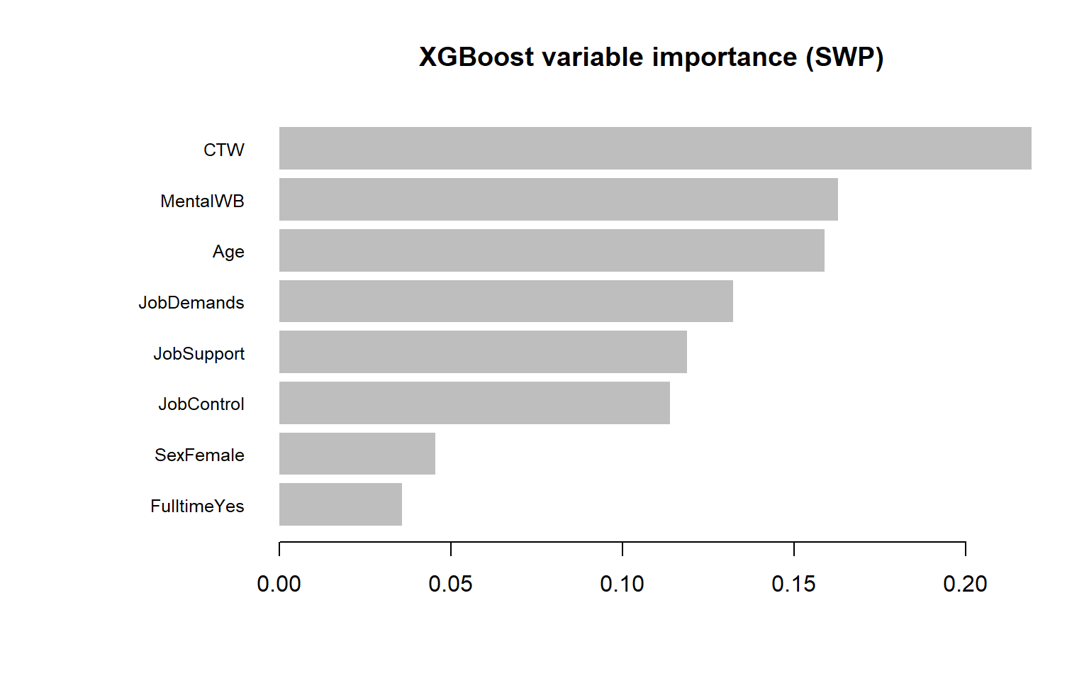
imp <- xgb.importance(feature_names = colnames(X_tr), model = xgb_fit)
xgb.plot.importance(imp, top_n = 8,
                    main = "XGBoost variable importance (SWP)")

4 Guided Practice

R is loading in the background — exercises below will be interactive once ready.

Tasks

Does XGBoost/gbm outperform random forest (C4) on test accuracy and sensitivity?
Compare variable importance — do the top predictors agree across methods?
Try lowering shrinkage to 0.01 and increasing trees to 500 — does it improve?

5 Why-Questions

Q: “Boosting, bagging, random forests — how do I choose?”

Rule of thumb: - Random forest: great default — parallelisable, robust, minimal tuning - Gradient boosting (XGBoost): often best performance, but requires tuning (learning rate, depth, rounds) and is sequential (slower) - Bagging: rarely used alone; superseded by random forests

In practice: try random forest first, then gradient boosting with early stopping if you need more accuracy. Both should be compared against the simpler methods (logistic, LASSO) — sometimes the gain is marginal and the simpler model is preferred for interpretability.