C7 — Calibration of Prediction Models

1 Concept: Does the Model’s Confidence Match Reality?

1.1 AUC tells you about ranking — calibration tells you about probabilities

A model with AUC = 0.85 ranks patients well: those with higher predicted probability tend to have the outcome more often. But a good AUC does not mean the probabilities are meaningful as numbers.

Calibration asks: if my model assigns probability 0.7 to a group of patients, do roughly 70% of them actually have the outcome?

A well-calibrated model: predicted probabilities match observed proportions
An overconfident model: probabilities close to 0 and 1, actual rates more moderate
An underconfident model: probabilities cluster near 0.5 even when outcomes are certain

Calibration is crucial for clinical decision-making. A model used to decide whether to screen a patient, prescribe a drug, or allocate an ICU bed must give meaningful probabilities — not just good rankings.

1.2 The calibration plot

The standard diagnostic is a calibration plot (also called a calibration curve):

Divide predicted probabilities into \(g\) groups (typically \(g = 10\) deciles)
For each group, compute the mean predicted probability and the observed event rate
Plot: x-axis = mean predicted probability, y-axis = observed proportion
A perfectly calibrated model falls on the diagonal

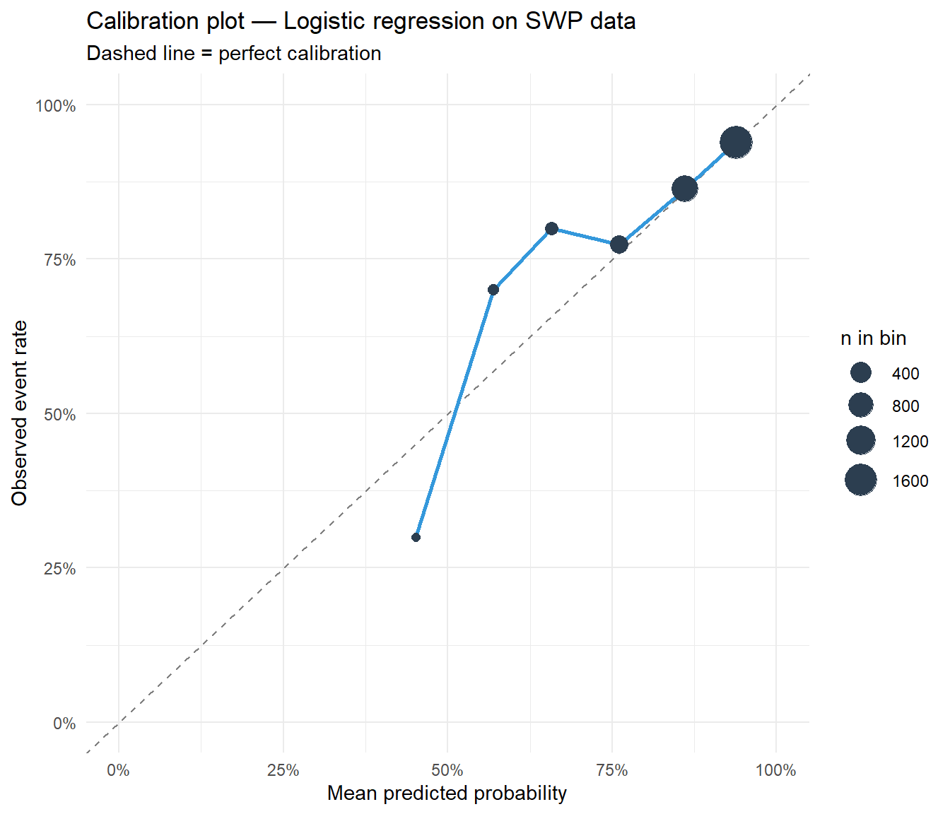
Points above the diagonal: observed rate exceeds prediction — model is underestimating risk. Points below the diagonal: observed rate below prediction — model is overestimating risk.

1.3 Hosmer–Lemeshow test

The Hosmer–Lemeshow (HL) test formally tests whether the calibration plot departs from the diagonal. It computes a chi-squared statistic over the \(g\) groups.

A large p-value (e.g. > 0.05): no evidence of miscalibration — observed and expected counts are close
A small p-value: significant miscalibration detected

Caveat: The HL test is sensitive to sample size. With large \(n\) it detects trivial departures; with small \(n\) it has low power. Always look at the calibration plot alongside the test.

2 Quiz

The model cannot rank patients by risk — its probability estimates are essentially random

Good discrimination but compressed probabilities — they do not reflect actual event rates

AUC and calibration always agree — any discrepancy signals a data processing error

The model has overfit the training data and cannot generalise to new patients

AUC measures discrimination: the probability that a randomly chosen case ranks above a randomly chosen control. It is unaffected by systematic shifts in the probability scale. A model that always predicts 0.4 ± 0.1 may discriminate well (the relative ordering is correct) but is miscalibrated (the absolute values are wrong). For decision-making — "should I screen this patient with predicted risk 0.6?" — calibration is essential.

The model assigns too-low probabilities to high-risk patients — it is underestimating

The model is overestimating risk here — it predicts 0.8 when the true observed rate is only 0.5

The model is perfectly calibrated — a predicted 0.8 matches the observed 0.8 event rate

The AUC must be poor — calibration failure necessarily implies poor discrimination too

If the calibration point (0.8, 0.5) is below the diagonal, the model overclaims certainty. Patients it calls "80% likely" are actually only 50% likely. This is common with tree-based methods (random forests, XGBoost) which can be overconfident in regions with few training observations. Logistic regression tends to be better calibrated by default; tree methods often require post-hoc recalibration (e.g. Platt scaling, isotonic regression).

The model is severely miscalibrated — p < 0.01 always warrants discarding the model

The model is well calibrated — p only needs to exceed 0.001 to confirm this

Significant, but n = 50 000 makes even tiny errors detectable — the calibration plot judges clinical relevance

The Hosmer-Lemeshow test is not valid for datasets with more than 10 000 observations

The HL test is a chi-squared test and gains power as n increases. With 50 000 observations, even a 2% deviation from the diagonal will be significant. A p-value of 0.002 does not tell you whether the miscalibration matters clinically. Always look at the calibration plot: if the curve hugs the diagonal with only small deviations, the model may still be clinically useful despite a significant HL test.

3 Worked Example: Calibration of a Logistic Regression Model on SWP Data

# Manual calibration plot using deciles of predicted probability
cal_df <- data.frame(
  pred = pred_glm,
  obs  = as.numeric(test$SWP)
)

# Cut into 10 equal-width bins
cal_df$bin <- cut(cal_df$pred, breaks = seq(0, 1, by = 0.1),
                  include.lowest = TRUE)

cal_summary <- cal_df |>
  group_by(bin) |>
  summarise(
    mean_pred = mean(pred),
    obs_rate  = mean(obs),
    n         = n(),
    .groups   = "drop"
  )

ggplot(cal_summary, aes(mean_pred, obs_rate)) +
  geom_abline(slope = 1, intercept = 0, linetype = "dashed", colour = "grey50") +
  geom_line(colour = "#3498db", linewidth = 1) +
  geom_point(aes(size = n), colour = "#2c3e50") +
  scale_size_continuous(range = c(2, 8), name = "n in bin") +
  scale_x_continuous(limits = c(0, 1), labels = scales::percent_format()) +
  scale_y_continuous(limits = c(0, 1), labels = scales::percent_format()) +
  labs(title = "Calibration plot — Logistic regression on SWP data",
       subtitle = "Dashed line = perfect calibration",
       x = "Mean predicted probability", y = "Observed event rate") +
  theme_minimal()

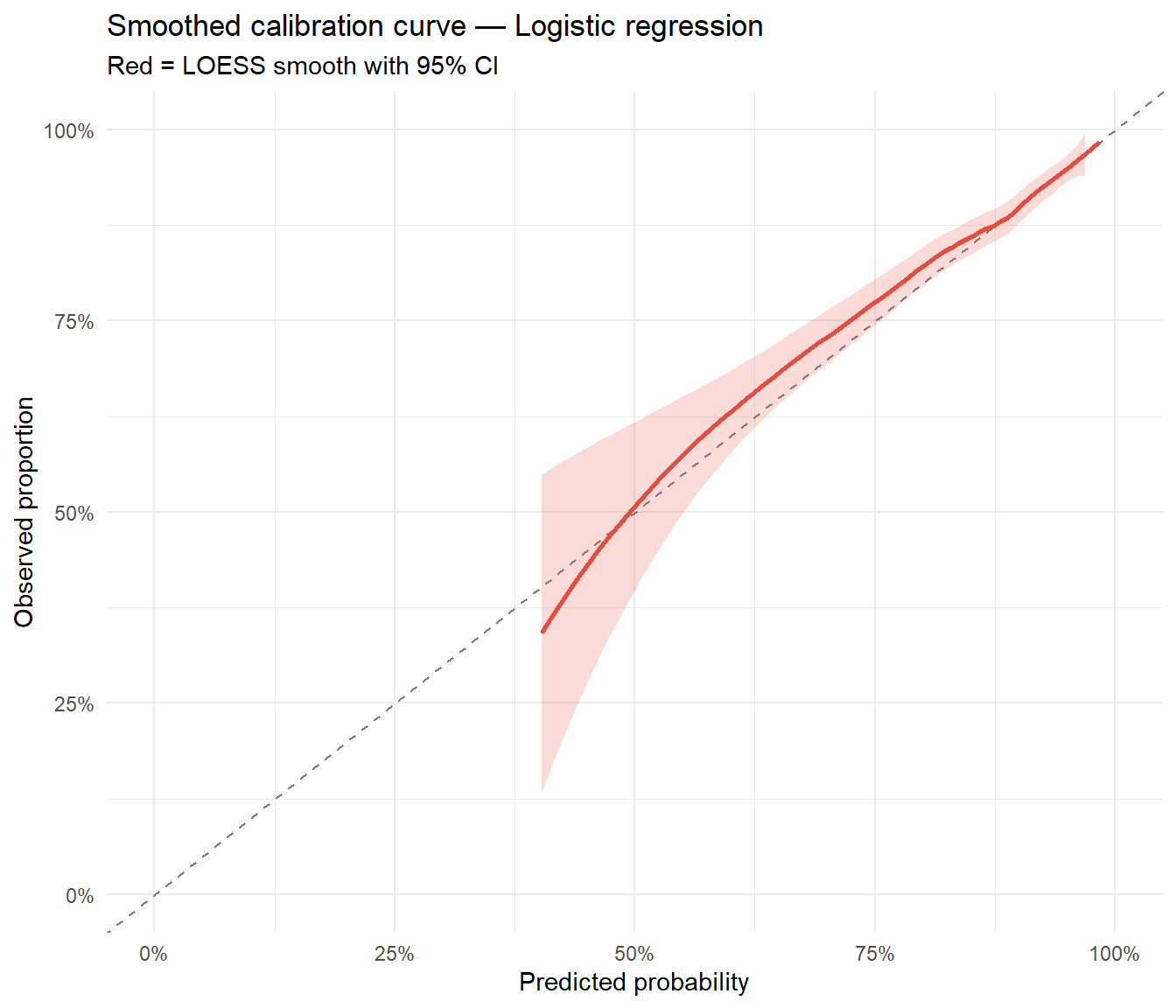
# Smoothed calibration curve using LOESS
ggplot(cal_df, aes(pred, obs)) +
  geom_abline(slope = 1, intercept = 0, linetype = "dashed", colour = "grey50") +
  geom_smooth(method = "loess", se = TRUE, colour = "#e74c3c",
              fill = "#e74c3c", alpha = 0.2) +
  scale_x_continuous(limits = c(0, 1), labels = scales::percent_format()) +
  scale_y_continuous(limits = c(0, 1), labels = scales::percent_format()) +
  labs(title = "Smoothed calibration curve — Logistic regression",
       subtitle = "Red = LOESS smooth with 95% CI",
       x = "Predicted probability", y = "Observed proportion") +
  theme_minimal()

`geom_smooth()` using formula = 'y ~ x'

# Hosmer-Lemeshow test (manual implementation without ResourceSelection)
hl_manual <- function(pred, obs, g = 10) {
  df   <- data.frame(pred, obs) |> arrange(pred)
  df$grp <- ntile(df$pred, g)
  tab  <- df |> group_by(grp) |>
    summarise(O1 = sum(obs), E1 = sum(pred),
              O0 = n() - sum(obs), E0 = n() - sum(pred), .groups = "drop")
  chi2 <- sum((tab$O1 - tab$E1)^2 / tab$E1 +
               (tab$O0 - tab$E0)^2 / tab$E0)
  p    <- 1 - pchisq(chi2, df = g - 2)
  cat(sprintf("Hosmer-Lemeshow chi2 = %.2f, df = %d, p = %.4f\n", chi2, g-2, p))
  invisible(list(chi2 = chi2, p = p))
}

hl_manual(pred_glm, as.numeric(test$SWP))

Hosmer-Lemeshow chi2 = 9.51, df = 8, p = 0.3010

4 Guided Practice

R is loading in the background — exercises will be interactive once the status bar disappears.

Hints

Points above the diagonal = observed rate exceeds prediction (underestimation)
Points below the diagonal = observed rate below prediction (overestimation)
Logistic regression is generally well-calibrated; tree-based methods often overestimate at extremes
A significant HL p-value does not automatically mean the model is unusable — inspect the plot

5 Retrieval Challenge

Model Answer

The naive model always predicts the marginal rate (a constant), so its calibration plot is a single point — trivially calibrated for that one probability value. The logistic regression spans the full probability range and its calibration curve should track the diagonal. AUC of the naive model is exactly 0.5 (random). This illustrates that a model can be “calibrated” in a trivial sense while having zero discrimination, and conversely a well-discriminating model may need recalibration.

6 Why-Questions

Q: “Tree-based models (random forests, XGBoost) often have poor calibration — why?”

Tree-based models output predicted probabilities that are leaf-node proportions (random forests average these across trees). In regions of the feature space with few training observations, leaf proportions are extreme (close to 0 or 1) even when the true probability is moderate. Logistic regression, by contrast, produces smooth probabilities governed by the linear predictor. Post-hoc recalibration methods like Platt scaling (logistic regression on the model outputs) or isotonic regression can correct tree-model calibration.

Q: “In the STA230 project, which is more important — AUC or calibration?”

It depends on the use case. For ranking patients on a risk score (triage, screening), AUC is the primary metric. For absolute risk estimates used in clinical decisions — “should we treat this patient with 40% predicted 5-year risk?” — calibration is essential. In the SWP project you fitted four models (logistic, CART, RF, XGBoost): compare both AUC and calibration to get a complete picture. A model with AUC = 0.82 and good calibration is more useful clinically than one with AUC = 0.85 but severely miscalibrated probabilities.

Q: “How does calibration relate to internal validation from the reading articles?”

The articles you read in Project 2 (Steyerberg et al., Harrell et al.) emphasise that optimism — the gap between apparent performance on training data and true performance on new data — affects both discrimination and calibration. Optimistic calibration appears as a calibration curve that is steeper than the diagonal (overconfident predictions). Internal validation via bootstrap or cross-validation corrects this optimism. The Hosmer–Lemeshow test on training data will always look better than on test data — always report calibration on held-out data.