U2 — K-Means Clustering

1 Concept: Finding Groups Without Labels

1.1 Supervised vs unsupervised — the key distinction

In Blocks 1 and 2 you always had a response variable Y: SBP to predict, disease to classify. Clustering has no Y. You observe $\mathbf{X}$ and ask: are there natural subgroups in this data?

In STA220 you asked a related question: do HAD items group into depression and anxiety? Factor analysis answered this by finding latent dimensions. Clustering answers a different version: do patients group into distinct health profiles? No labels are assumed — the groups emerge from the data geometry.

1.2 The k-means algorithm

Given $n$ observations and a chosen number of clusters $K$, k-means minimises the total within-cluster sum of squares (WCSS):

\[\text{WCSS} = \sum_{k=1}^{K} \sum_{i \in C_k} \|\mathbf{x}_i - \boldsymbol{\mu}_k\|^2\]

where $\boldsymbol{\mu}_k$ is the centroid (mean) of cluster $k$.

Algorithm (Lloyd’s):

Randomly initialise $K$ centroids
Assign each observation to the nearest centroid
Update each centroid as the mean of its assigned observations
Repeat steps 2–3 until assignments stop changing

The algorithm converges to a local minimum — not necessarily the global minimum. Always run with multiple random starts (nstart in R) and take the best result.

1.3 Choosing K — the elbow method

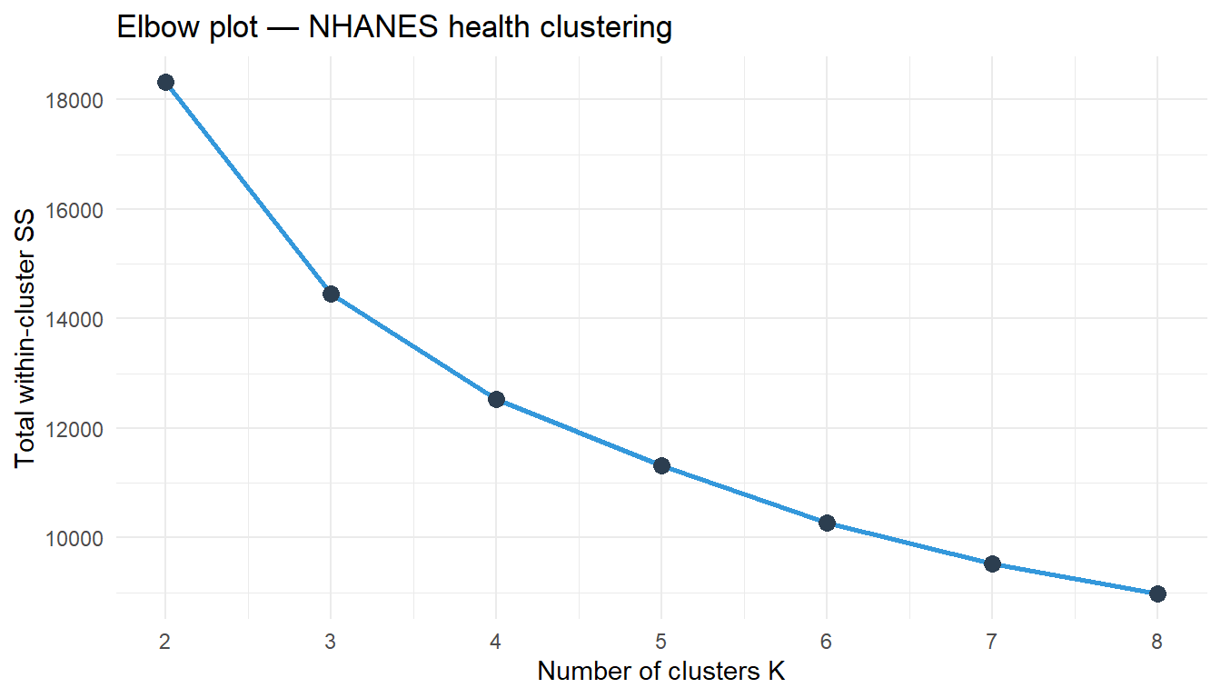
Run k-means for $K = 1, 2, \ldots, K_{\max}$ and plot WCSS against $K$. WCSS always decreases as $K$ increases (more clusters = smaller groups = tighter fit). Look for an elbow — the point where the rate of decrease slows sharply.

There is no objectively correct $K$. Domain knowledge matters: do you expect 2 patient profiles or 5? The elbow is a heuristic, not a rule.

1.4 Important: scale your variables

K-means uses Euclidean distance. If Age is measured in years (range 20–80) and Cholesterol in mmol/L (range 2–8), Age will dominate purely because of its larger scale. Always standardise before clustering.

2 Quiz

Clusters that are maximally separated from each other in space

Observations within each cluster are close to their centroid — compact and tightly grouped

Clusters of approximately equal size across all groups

Clusters whose observations follow a multivariate normal distribution

WCSS penalises observations that are far from their cluster centroid. Minimising WCSS makes clusters internally compact. It does not directly maximise between-cluster distance, though the two are related. Equal-size clusters and normality are not required — but k-means performs poorly when clusters are very unequal in size or non-spherical in shape.

k-means is inherently stochastic and cluster assignments never converge to any stable configuration

Random starting centroids lead to different local minima and different final cluster assignments

k-means randomly resamples the input data before each run, causing the cluster geometry to change

k-means requires at least K ≥ 5 clusters for the algorithm to converge to a reproducible assignment

With nstart = 1, k-means starts from one random set of centroids. Different starting points lead to different local minima. Always use nstart ≥ 20 and set.seed() for reproducibility. R's kmeans() returns the best result across all starts (lowest WCSS).

K-means cannot process four variables simultaneously — it is restricted to working with only two dimensions

K-means automatically forms perfectly spherical, equal-volume clusters regardless of variable scale

Large-scale SBP dominates Euclidean distance — clusters reflect blood pressure above all other variables

The algorithm will cycle indefinitely between inconsistent cluster assignments and never converge

Euclidean distance treats all dimensions equally in units. SBP (range ~110) contributes 110² ≈ 12000 to squared distance per unit change; BMI (range ~35) contributes 35² ≈ 1225. SBP numerically dominates. Standardise first so each variable has mean 0 and SD 1, giving equal weight to all variables.

3 Worked Example: Patient Health Profiles in NHANES

We cluster NHANES patients into groups based on their health profile — no outcome variable used.

set.seed(42)
vars <- c("Age", "BMI", "Waist", "Cholesterol", "SBP")
dat  <- na.omit(nhanes[, vars])
X    <- scale(dat)

# Run k-means for K = 2 to 8, record WCSS
wcss <- sapply(2:8, function(k) {
  kmeans(X, centers = k, nstart = 25)$tot.withinss
})

Warning: did not converge in 10 iterations

data.frame(K = 2:8, WCSS = wcss)

  K      WCSS
1 2 18324.019
2 3 14448.161
3 4 12524.371
4 5 11317.832
5 6 10270.836
6 7  9517.159
7 8  8971.919

ggplot(data.frame(K = 2:8, WCSS = wcss), aes(K, WCSS)) +
  geom_line(colour = "#3498db", linewidth = 1) +
  geom_point(size = 3, colour = "#2c3e50") +
  scale_x_continuous(breaks = 2:8) +
  labs(title = "Elbow plot — NHANES health clustering",
       x = "Number of clusters K", y = "Total within-cluster SS") +
  theme_minimal()

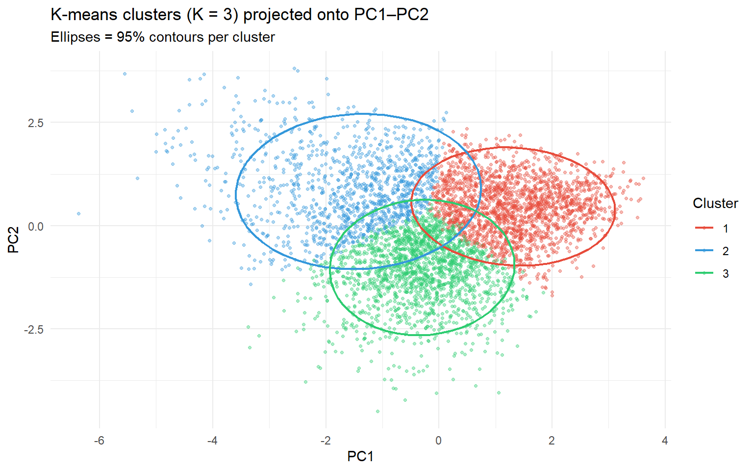
set.seed(42)
km3 <- kmeans(X, centers = 3, nstart = 25)
dat$cluster <- factor(km3$cluster)

# Cluster means (back on original scale)
aggregate(dat[, vars], by = list(Cluster = dat$cluster), FUN = mean) |>
  mutate(across(where(is.numeric), round, 1))

Warning: There was 1 warning in `mutate()`.
ℹ In argument: `across(where(is.numeric), round, 1)`.
Caused by warning:
! The `...` argument of `across()` is deprecated as of dplyr 1.1.0.
Supply arguments directly to `.fns` through an anonymous function instead.

  # Previously
  across(a:b, mean, na.rm = TRUE)

  # Now
  across(a:b, \(x) mean(x, na.rm = TRUE))

  Cluster  Age  BMI Waist Cholesterol   SBP
1       1 33.5 25.2  87.6       177.9 112.7
2       2 47.0 38.6 121.1       183.8 126.0
3       3 63.3 27.6  98.2       205.0 136.1

# Visualise clusters on first two PCs
pca <- prcomp(X)
scores <- data.frame(pca$x[, 1:2], cluster = dat$cluster)

ggplot(scores, aes(PC1, PC2, colour = cluster)) +
  geom_point(alpha = 0.4, size = 0.9) +
  stat_ellipse(linewidth = 0.8) +
  scale_colour_manual(values = c("#e74c3c", "#3498db", "#2ecc71")) +
  labs(title = "K-means clusters (K = 3) projected onto PC1–PC2",
       subtitle = "Ellipses = 95% contours per cluster",
       colour = "Cluster") +
  theme_minimal()

Interpretation: Three clusters emerge — broadly: younger healthy, middle-aged overweight, older hypertensive. These are data-driven profiles, not clinical diagnoses. The PC projection shows how well-separated the clusters are in the low-dimensional space found by PCA.

4 Guided Practice

R is loading in the background — exercises will be interactive once the status bar disappears.

Hints

kmeans(X, centers = K, nstart = 25)$tot.withinss gives WCSS for a given K
Use aggregate() or group_by() |> summarise() to get cluster means
Look at each cluster’s mean Age, BMI, and SBP to give it a clinical label
There is no “correct” label — interpretation requires domain knowledge

5 Retrieval Challenge

Model Answer

library(ggplot2)
ggplot(dat2, aes(BMI, SBP, colour = cluster)) +
  geom_point(alpha = 0.3, size = 0.7) +
  stat_ellipse() +
  scale_colour_manual(values = c("#e74c3c", "#3498db", "#2ecc71")) +
  labs(title = "K-means (K=3) on BMI and SBP only") +
  theme_minimal()
# Compare: are the 2-variable clusters similar to the 5-variable clusters?
# What information is lost by ignoring Age, Waist, Cholesterol?

6 Why-Questions

Q: “Is cluster 1 really different from cluster 2? Maybe they just look different by chance.”

K-means always produces K clusters — even on completely random data. There is no built-in test for whether clusters are “real”. One approach: compare the WCSS improvement from K-1 to K against the same step in randomly permuted data (the gap statistic). Another: check if the cluster structure replicates in a held-out half of the data. In practice, assess clusters on clinical interpretability, not just WCSS.

Q: “K-means gave my colleague different clusters on the same data. Is one of us wrong?”

Not necessarily. K-means can find different local optima on the same data, especially when clusters are not well-separated. Both solutions may be valid local minima. Solutions: (1) use set.seed() for reproducibility, (2) use nstart = 25 or more, (3) if results are very sensitive to initialisation, consider hierarchical clustering (next page) which is deterministic.

Q: “Can I use K-means to validate the factor structure I found in STA220?”

Not directly — k-means clusters observations (patients), while factor analysis clusters variables (HAD items). But you can use PCA scores as input to k-means: run PCA on the HAD items → take the first two PC scores → run k-means on patients in that 2D space. Patients who score similarly on both the depression and anxiety dimensions will cluster together. This bridges the two methods.