Lowest variance among all linear unbiased estimators
Lowest bias among all estimators
Highest R² on training data
Gauss-Markov: among estimators of the form β̂ = Cy (linear in Y) that are unbiased (E[β̂] = β), OLS has minimum variance. But 'best' is restricted to this class. A biased estimator (Ridge, LASSO) can have lower MSE if the variance reduction outweighs the bias introduced — exactly the bias-variance tradeoff.
Both training R² and test MSE decrease
Training R² decreases, test MSE increases
Training R² stays the same or increases; test MSE increases
Both stay the same since the predictors are irrelevant
Adding any predictor (even pure noise) can only increase or maintain training R² — OLS finds a non-zero coefficient that fits the training noise. On test data those noise coefficients hurt. Training fit improves, generalisation worsens — the classic overfitting pattern.
Normality of residuals
Independence of observations
Linearity — the true relationship is non-linear
Homoskedasticity — variance changes with fitted values
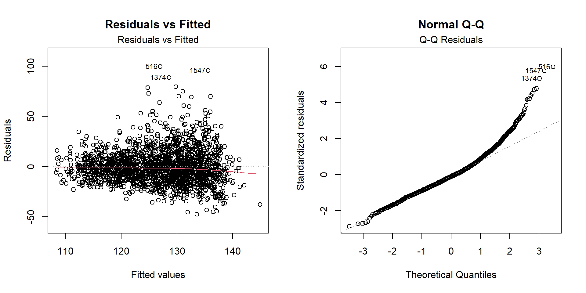
A U-shape (systematic curve) in residuals vs fitted means the model consistently over- or underpredicts in certain ranges — a sign of non-linearity. A funnel shape (widening spread) would indicate heteroskedasticity instead. Both can appear together.
3 Worked Example: Predicting Systolic Blood Pressure (NHANES)
The dataset is NHANES 2015–2016 (n = 5 005 adults). Outcome: mean systolic blood pressure (SBP, mmHg). Predictors: age, sex, BMI, waist circumference, total cholesterol, diabetes, smoking status.
fit <-lm(SBP ~ Age + Sex + BMI + Waist + Cholesterol +factor(Diabetes) +factor(Smoker),data = nhanes)summary(fit)
Call:
lm(formula = SBP ~ Age + Sex + BMI + Waist + Cholesterol + factor(Diabetes) +
    factor(Smoker), data = nhanes)

Residuals:
    Min      1Q  Median      3Q     Max
-47.574 -10.560  -1.809   8.120  99.653

Coefficients:
                   Estimate Std. Error t value Pr(>|t|)
(Intercept)       93.140206   3.226871  28.864  < 2e-16 ***
Age                0.410620   0.025722  15.964  < 2e-16 ***
SexMale            3.055668   0.821634   3.719 0.000206 ***
BMI                0.460422   0.153106   3.007 0.002670 **
Waist             -0.095662   0.063598  -1.504 0.132702
Cholesterol        0.030336   0.008705   3.485 0.000503 ***
factor(Diabetes)1  1.083909   1.072427   1.011 0.312281
factor(Smoker)1    1.988412   0.792813   2.508 0.012220 *
---
Signif. codes:  0 '***' 0.001 '**' 0.01 '*' 0.05 '.' 0.1 ' ' 1

Residual standard error: 16.64 on 1978 degrees of freedom
  (3019 observations deleted due to missingness)
Multiple R-squared:  0.1558,    Adjusted R-squared:  0.1528
F-statistic: 52.16 on 7 and 1978 DF,  p-value: < 2.2e-16
par(mfrow =c(1, 2))plot(fit, which =1, main ="Residuals vs Fitted")plot(fit, which =2, main ="Normal Q-Q")
R is loading in the background — the exercises below will be interactive once the status bar disappears.
TipWhat to look for
Does the full model have lower training RMSPE than the small model?
Does it also have lower test RMSPE? How large is the optimism gap?
Clinically: how precise are these predictions in mmHg? Is the model useful?
5 Retrieval Challenge
6 Why-Questions
CautionQ: “Both BMI and waist circumference are in the model. Is that OK?”
Both measure adiposity and are strongly correlated — this is multicollinearity. Including both inflates their standard errors, making individual coefficients less reliable. Options: (1) include only one (waist is often preferred as it captures central adiposity better), (2) use PCA to create a composite, (3) use Ridge/LASSO which handle multicollinearity automatically. For prediction, multicollinearity is less of a problem than for inference.
CautionQ: “My RMSPE is 17 mmHg. Is that a good model?”
It depends on context. A clinically meaningful difference in SBP is typically 5–10 mmHg. An RMSPE of 17 mmHg means individual predictions are off by ~17 mmHg on average — likely too imprecise for individual-level clinical decisions. However, the model may still be useful for population-level inference about which factors are associated with SBP. Precision and interpretability are separate goals.
NoteFurther reading
James et al. (2021). An Introduction to Statistical Learning. — Chapter 3