C3 — Decision Trees (CART)

1 Concept: Recursive Partitioning

1.1 How CART works

A classification tree recursively splits the predictor space into rectangular regions. At each node, it finds the predictor \(X_j\) and split point \(s\) that minimises the Gini impurity in the resulting child nodes:

\[G = \sum_{k} \hat{p}_{mk}(1 - \hat{p}_{mk})\]

where \(\hat{p}_{mk}\) is the proportion of class \(k\) observations in region \(m\). \(G=0\) means a pure node (all one class); \(G=0.5\) is maximally impure for a binary outcome.

1.2 Pruning to avoid overfitting

A fully grown tree overfits — it memorises the training data. Cost-complexity pruning adds a penalty \(\alpha \cdot |\text{leaves}|\) to the tree size. The optimal \(\alpha\) is found by cross-validation.

1.3 Strengths and weaknesses

Strength	Weakness
Interpretable — easy to visualise	High variance — small data changes give different trees
Handles mixed variable types naturally	Usually outperformed by ensemble methods
Captures interactions automatically	Axis-aligned splits only
No need to standardise	Prone to overfitting without pruning

2 Quiz

0.90

0.10

0.18 (= 0.9×0.1 + 0.1×0.9)

0.50

Gini = Σ p_k(1−p_k) = 0.9×0.1 + 0.1×0.9 = 0.18. A pure node (all one class) has G=0. A completely mixed node (50/50 binary) has G=0.5. The tree algorithm searches for splits that most reduce G — it prefers splits that create pure child nodes.

They consider all p predictors at each split, which inflates variance dramatically

A single different observation can flip an early split and restructure the entire tree below it

The Gini criterion amplifies the effect of outliers at every split

Pruning introduces bias that destabilises the remaining tree structure

Trees are hierarchical: the first split affects all subsequent splits. If a slightly different training set causes a different top-level split, the entire tree changes. This makes trees unstable — high variance. Random forests fix this by averaging many trees grown on bootstrap samples, dramatically reducing variance while keeping the bias low.

Grows a deeper, more complex tree

Prunes more aggressively — produces a smaller, simpler tree

Changes the splitting criterion from Gini to entropy

Increases the minimum number of observations required per leaf

cp is the minimum improvement in fit required to add a split. Higher cp → harder to improve enough → fewer splits → smaller tree. Setting cp=0 grows the full tree (maximum overfit). The optimal cp is found by CV — rpart's plotcp() shows cross-validated error vs cp, and you pick the cp at the minimum (or within 1 SE of it).

3 Worked Example

library(rpart)

tree_full <- rpart(SWP ~ Age + Sex + Fulltime + CTW + JobDemands +
                     JobControl + JobSupport + MentalWB + DemandCtrl,
                   data = train, method = "class",
                   control = rpart.control(cp = 0.001, minsplit = 20))

printcp(tree_full)


Classification tree:
rpart(formula = SWP ~ Age + Sex + Fulltime + CTW + JobDemands + 
    JobControl + JobSupport + MentalWB + DemandCtrl, data = train, 
    method = "class", control = rpart.control(cp = 0.001, minsplit = 20))

Variables actually used in tree construction:
[1] Age        CTW        DemandCtrl Fulltime   JobControl JobDemands JobSupport
[8] MentalWB   Sex       

Root node error: 786/7000 = 0.11229

n= 7000 

          CP nsplit rel error  xerror     xstd
1  0.0045802      0   1.00000 1.00000 0.033607
2  0.0042409      5   0.97710 0.99237 0.033494
3  0.0038168     14   0.93384 0.99237 0.033494
4  0.0036896     22   0.90331 0.97710 0.033268
5  0.0033927     32   0.86641 0.96692 0.033115
6  0.0025445     38   0.84606 0.97328 0.033211
7  0.0021204     40   0.84097 0.97583 0.033249
8  0.0020356     44   0.83079 0.97710 0.033268
9  0.0019084     49   0.82061 0.97328 0.033211
10 0.0017812     71   0.77481 0.99237 0.033494
11 0.0015267     76   0.76590 0.99618 0.033551
12 0.0012723     82   0.75573 0.99364 0.033513
13 0.0010000    105   0.72392 0.99873 0.033588

# Prune at optimal cp (1-SE rule)
cp_opt <- tree_full$cptable[which.min(tree_full$cptable[,"xerror"]), "CP"]
tree_pruned <- prune(tree_full, cp = cp_opt)

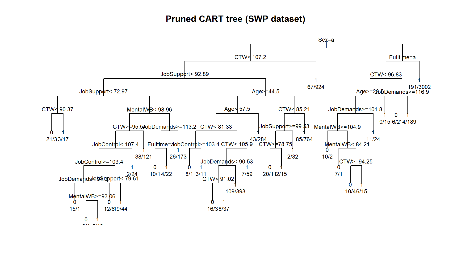
plot(tree_pruned, uniform = TRUE, main = "Pruned CART tree (SWP dataset)")
text(tree_pruned, use.n = TRUE, cex = 0.75)

pred_class <- predict(tree_pruned, newdata = test, type = "class")
cm <- table(Predicted = pred_class, Actual = test$SWP)
print(cm)

         Actual
Predicted    0    1
        0   28   20
        1  289 2663

cat("\nTest accuracy:      ", round(mean(pred_class == test$SWP)*100, 1), "%\n")


Test accuracy:       89.7 %

cat("Sensitivity (SWP=0):", round(cm[1,1]/sum(cm[,1])*100, 1), "%\n")

Sensitivity (SWP=0): 8.8 %

cat("Specificity (SWP=1):", round(cm[2,2]/sum(cm[,2])*100, 1), "%\n")

Specificity (SWP=1): 99.3 %

# Variable importance
cat("\nVariable importance:\n")


Variable importance:

print(round(sort(tree_pruned$variable.importance, decreasing=TRUE), 1))

       CTW JobSupport JobDemands   MentalWB   Fulltime        Age        Sex 
      90.3       51.3       37.0       29.1       28.3       28.0       22.1 
DemandCtrl JobControl 
      21.7       21.0

4 Guided Practice

R is loading in the background — exercises below will be interactive once ready.

What to look for

The top split predictor is the single most informative variable for SWP
Compare to CTW, MentalWB, JobControl — which one dominates?
Does the deep tree have lower test accuracy than the shallow one? (Overfitting)

5 Why-Questions

Q: “The tree is interpretable but random forests are better. When would I still use a single tree?”

Single trees are useful when: (1) you need to explain the decision logic to non-technical stakeholders (a tree can be printed as a flowchart), (2) you have regulatory constraints requiring transparent decisions (e.g., clinical triage rules), (3) the dataset is very small and ensemble methods overfit. For pure prediction, random forests almost always outperform single trees.