U3 — Hierarchical Clustering

1 Concept: A Tree of Clusters

1.1 Why hierarchical clustering?

K-means requires you to choose \(K\) before you start. Hierarchical clustering builds a tree (dendrogram) that shows the nested cluster structure at every level — you choose \(K\) after seeing the tree. It is also deterministic: the same data always gives the same result, unlike k-means.

A second advantage: the dendrogram reveals how clusters relate to each other. Are clusters 1 and 2 more similar to each other than to cluster 3? The tree shows this immediately.

1.2 Bottom-up (agglomerative) clustering

The most common approach:

Start with \(n\) clusters — every observation is its own cluster
Merge the two most similar clusters
Repeat until all observations are in one cluster

The result is a dendrogram. To get \(K\) clusters, cut the tree at height \(h\) such that exactly \(K\) branches extend below the cut.

1.3 Linkage — how similarity is measured between clusters

Once clusters contain multiple observations, we need to define distance between clusters (not just individual points).

Linkage	Distance between clusters A and B
Complete	Maximum distance between any point in A and any point in B
Single	Minimum distance (nearest neighbours)
Average	Average distance between all pairs
Ward’s	Increase in total WCSS when merging A and B

Ward’s linkage is usually recommended for health data — it produces compact, similarly sized clusters and connects directly to k-means (both minimise WCSS).

1.4 Reading a dendrogram

Height of a merge = dissimilarity at which two clusters joined
Long vertical lines = large gap between levels = natural cluster boundary
Short lines = clusters joined at similar dissimilarity = less clear separation
Cut the tree where you see the longest vertical lines before the cut

2 Quiz

Hierarchical clustering guarantees the globally optimal cluster assignment at every level of the tree

Hierarchical clustering always runs faster than k-means, regardless of dataset size or dimensionality

K is not specified upfront — the dendrogram shows structure at all levels and K is chosen after viewing it

Hierarchical clustering requires no standardisation because it adjusts for variable scale automatically

K-means requires K as input. Hierarchical clustering builds a full tree and you choose K by deciding where to cut the dendrogram — after seeing the structure. This is useful when you have no prior expectation about the number of groups. Hierarchical clustering still requires standardisation and a choice of linkage method, so it is not assumption-free.

Very elongated chain-like clusters that grow by absorbing nearby points one at a time

Compact, roughly spherical clusters — merging only when even the most distant points are still close

Clusters that are forced to contain exactly the same number of observations

Clusters that always reproduce k-means output with the same K

Complete linkage is conservative: two clusters only merge if their most distant members are still close enough. This prevents one large loose cluster from absorbing everything (the "chaining" problem of single linkage). The result is compact, roughly spherical clusters. Ward's linkage is similar in spirit but uses WCSS as the criterion.

Heights 4.2 and 0.8 indicate the number of observations present in each cluster when it is formed

Merge height equals dissimilarity — the large gap from 0.8 to 4.2 signals a natural cluster boundary

Equal heights across all merges is required — unequal values indicate a bug in the linkage calculation

Higher merge height indicates a better, more clearly defined cluster with stronger internal homogeneity

Height in a dendrogram = the dissimilarity (e.g. Euclidean distance) at which the merge happened. A large height means the two clusters were far apart before merging — cutting the tree just below this height preserves the separation. Long vertical lines in a dendrogram indicate natural boundaries. Short lines indicate clusters that were already very similar.

3 Worked Example: Hierarchical Clustering of NHANES Patients

vars <- c("Age", "BMI", "Waist", "Cholesterol", "SBP")
set.seed(42)
# Use a subsample of 300 for readable dendrogram
idx  <- sample(which(complete.cases(nhanes[, vars])), 300)
dat  <- nhanes[idx, vars]
X    <- scale(dat)

# Compute Euclidean distance matrix
dist_X <- dist(X, method = "euclidean")

# Fit hierarchical clustering with Ward's linkage
hc <- hclust(dist_X, method = "ward.D2")

plot(hc, labels = FALSE, hang = -1,
     main = "Dendrogram — NHANES health variables (Ward's linkage)",
     xlab = "Patients", ylab = "Height (dissimilarity)")
abline(h = 12, col = "#e74c3c", lty = 2, lwd = 1.5)
legend("topright", legend = "Cut at h = 12 → 3 clusters",
       col = "#e74c3c", lty = 2, bty = "n")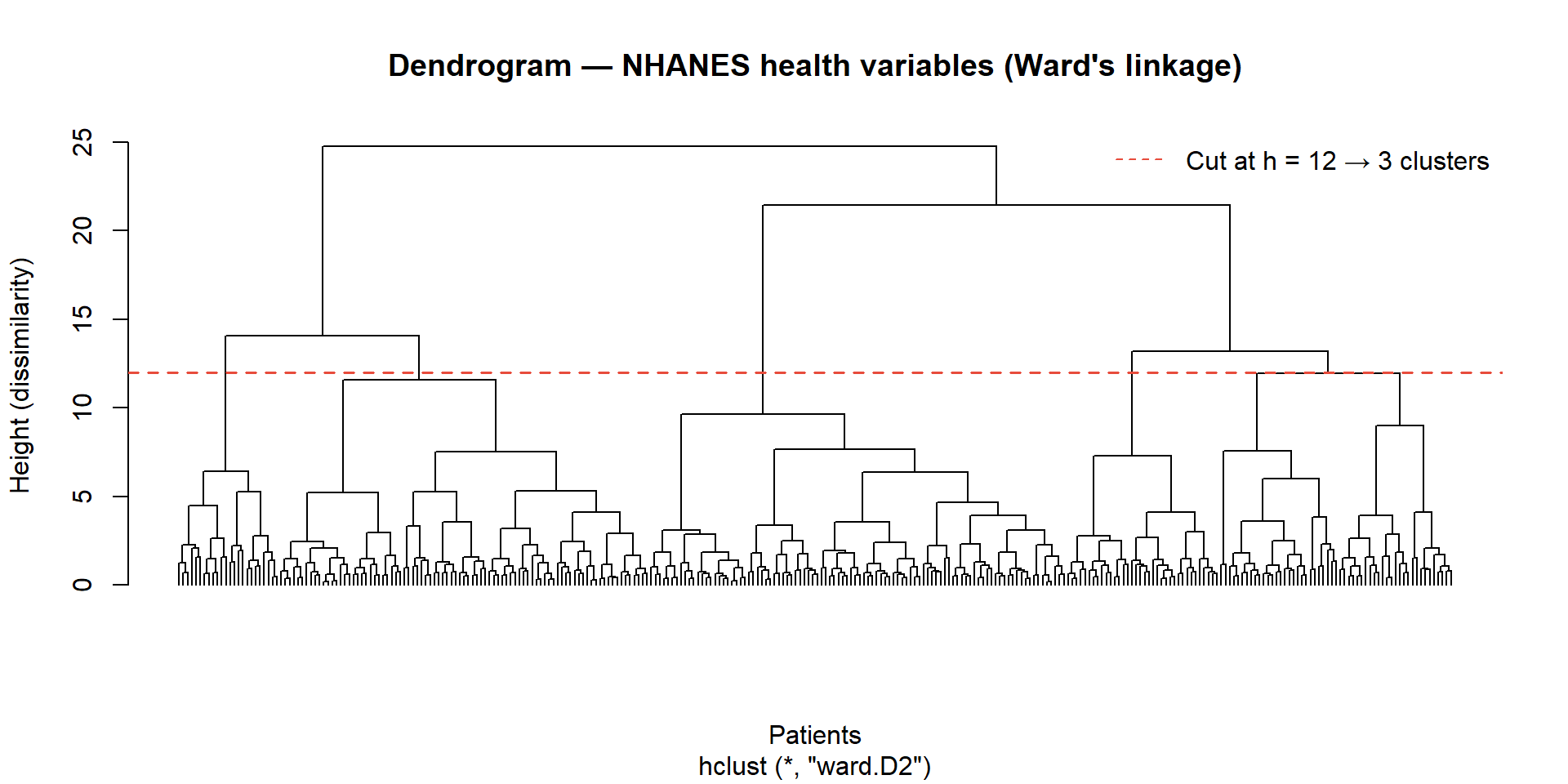

# Cut at K = 3
clusters <- cutree(hc, k = 3)
dat$cluster <- factor(clusters)

# Cluster means
aggregate(dat[, vars], by = list(Cluster = dat$cluster), FUN = mean) |>
  mutate(across(where(is.numeric), round, 1))

Warning: There was 1 warning in `mutate()`.
ℹ In argument: `across(where(is.numeric), round, 1)`.
Caused by warning:
! The `...` argument of `across()` is deprecated as of dplyr 1.1.0.
Supply arguments directly to `.fns` through an anonymous function instead.

  # Previously
  across(a:b, mean, na.rm = TRUE)

  # Now
  across(a:b, \(x) mean(x, na.rm = TRUE))

  Cluster  Age  BMI Waist Cholesterol   SBP
1       1 47.4 35.9 114.5       184.7 123.0
2       2 32.5 25.2  87.2       182.6 114.0
3       3 62.2 26.3  94.2       213.4 133.5

pca <- prcomp(X)
scores <- data.frame(pca$x[, 1:2], cluster = dat$cluster)

ggplot(scores, aes(PC1, PC2, colour = cluster)) +
  geom_point(alpha = 0.5, size = 1.2) +
  stat_ellipse(linewidth = 0.8) +
  scale_colour_manual(values = c("#e74c3c", "#3498db", "#2ecc71")) +
  labs(title = "Hierarchical clusters (K = 3, Ward's) on PC1–PC2",
       colour = "Cluster") +
  theme_minimal()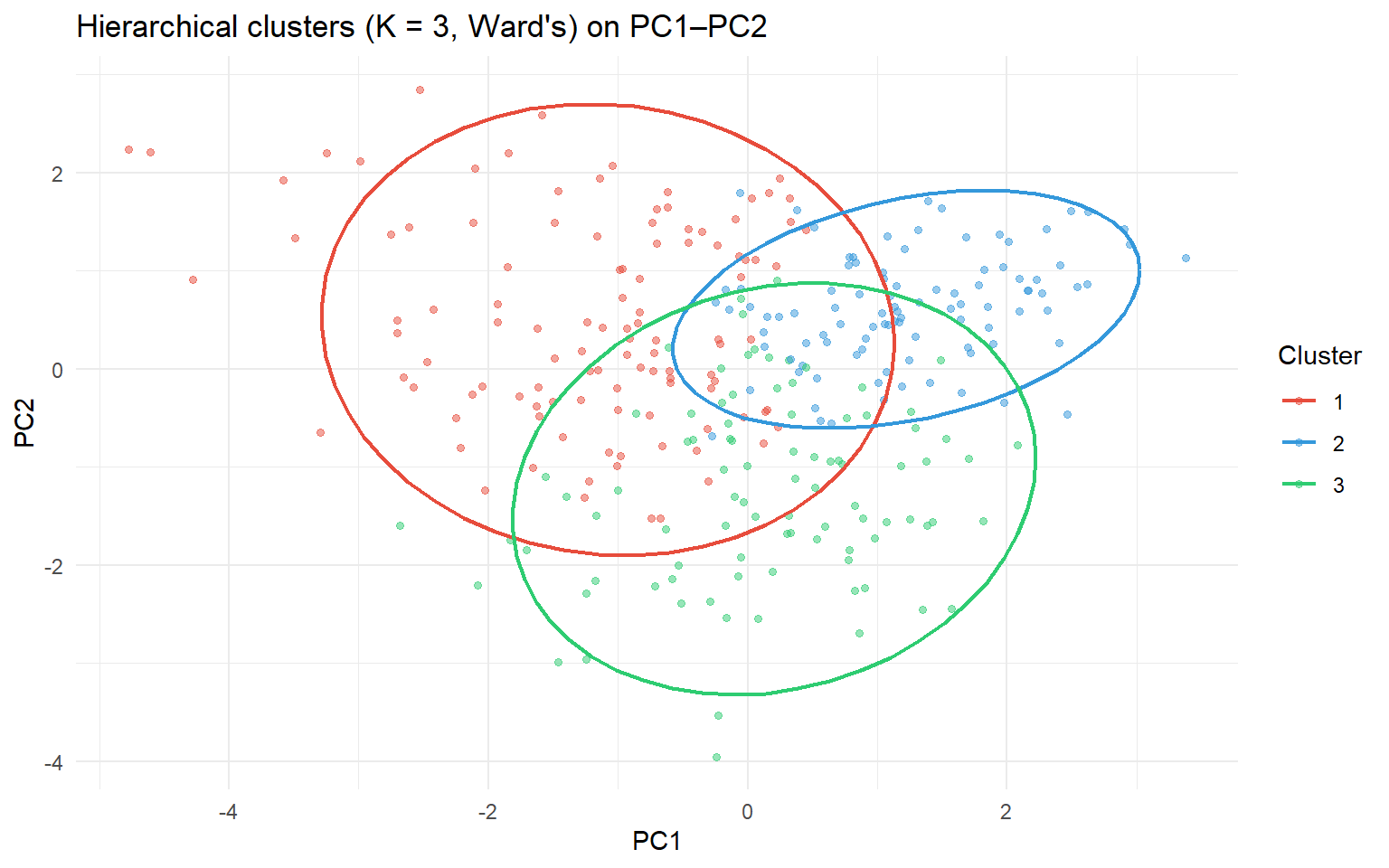

Comparing to k-means: Ward’s hierarchical clustering often produces similar results to k-means because both minimise WCSS. The key difference: hierarchical clustering is deterministic and shows the full tree; k-means is faster on large datasets.

4 Guided Practice

R is loading in the background — exercises will be interactive once the status bar disappears.

Hints

hclust(dist(X), method = "ward.D2") for Ward’s linkage
cutree(hc, k = 3) to cut the tree into 3 clusters
table(cutree(hc, k = K)) shows how many observations per cluster
Ward’s tends to give more balanced cluster sizes than complete or single linkage

5 Retrieval Challenge

Model Answer

pca    <- prcomp(X)
scores <- pca$x[, 1:2]          # Keep first 2 PCs

D_pc   <- dist(scores)
hc_pc  <- hclust(D_pc, method = "ward.D2")
plot(hc_pc, labels = FALSE, hang = -1, main = "Clustering on PC1–PC2")

cl <- cutree(hc_pc, k = 3)
df <- data.frame(scores, cluster = factor(cl))

library(ggplot2)
ggplot(df, aes(PC1, PC2, colour = cluster)) +
  geom_point(alpha = 0.5) +
  stat_ellipse() +
  theme_minimal() +
  labs(title = "Hierarchical clusters on PC scores")
# Note: clustering on 2 PCs discards ~30% of variance vs full 5-variable clustering

6 Why-Questions

Q: “Should I use k-means or hierarchical clustering?”

Use hierarchical when: you don’t know K, you want to see the full tree structure, the dataset is small enough for a readable dendrogram (n < ~1000), or reproducibility matters. Use k-means when: n is large (k-means is O(nKd) per iteration, hclust is O(n² log n)), you have a strong prior on K, or you need to re-cluster new observations (you can assign new points to the nearest centroid in k-means). For health data at master’s level, hierarchical with Ward’s linkage is usually the starting point.

Q: “How does this connect to what I did with factor analysis in STA220?”

Factor analysis (FA) and clustering both reveal structure in unlabelled data. FA finds latent dimensions in the variable space — the HAD items cluster into depression and anxiety constructs. Hierarchical clustering finds groups in the observation space — patients group into health profiles. You can chain them: run FA to find the latent dimensions (or use PCA), then use the factor scores (or PC scores) as input to clustering. This gives clusters that are defined by the latent structure, not by the raw item correlations.

Q: “The dendrogram looks like two large groups at the top but K = 3 seems better from the elbow plot. Which do I trust?”

Use both sources of evidence. The dendrogram shows the hierarchical structure; the elbow plot (from k-means) shows WCSS. If the dendrogram shows two very clear top-level groups and one of them splits into two sub-groups at a lower height, K = 3 is a natural choice — two main profiles, one of which has two subtypes. There is no single correct K; describe what you find at multiple levels and let the research question guide the final choice.