F3 — Training vs Test Error

1 Concept: Why Training Error is Optimistic

1.1 Optimism of training error

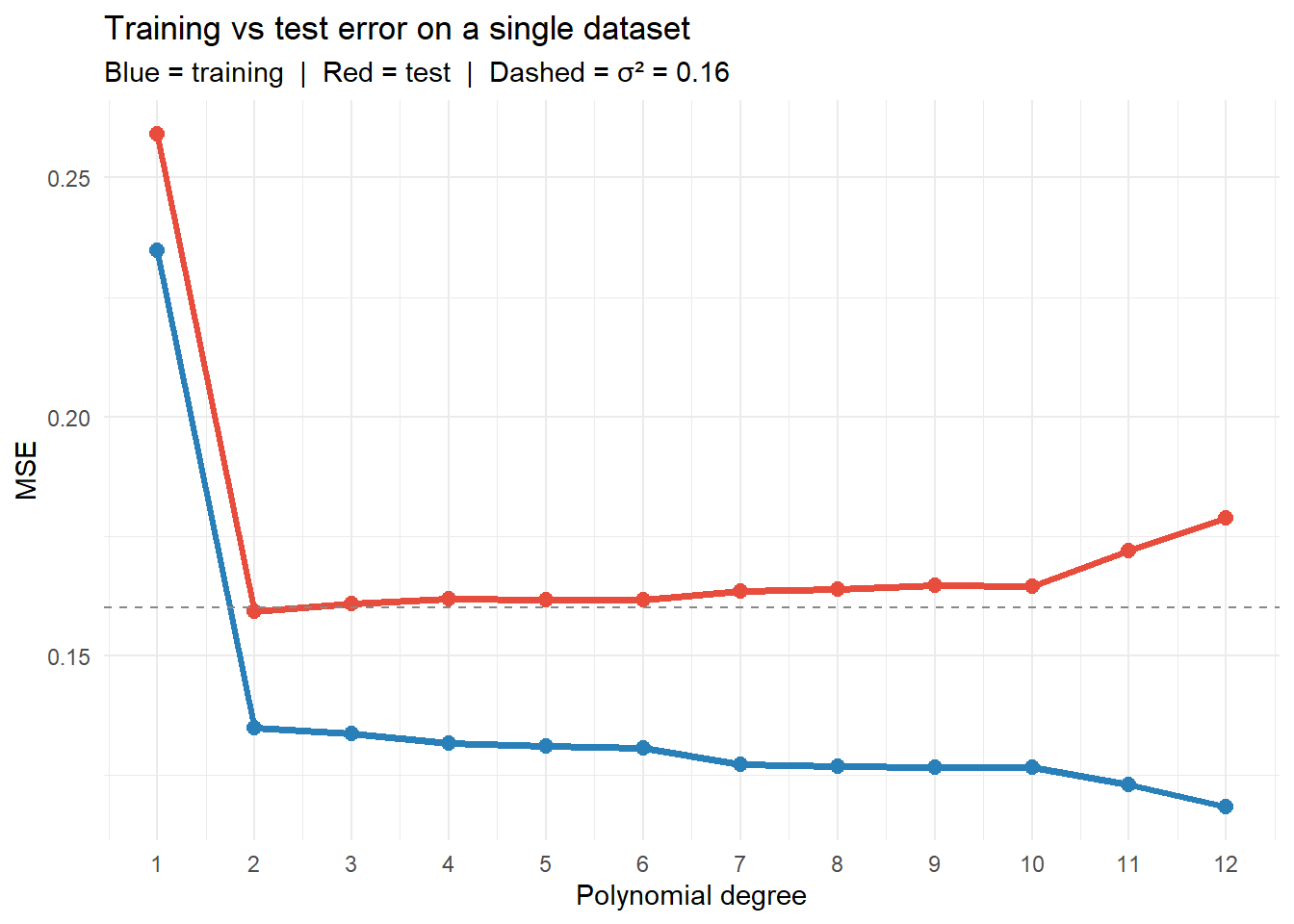
When we fit \(\hat{f}\) on training data and then evaluate on the same data, the estimate is optimistically biased. The model has already adapted to the specific noise in the training set.

The expected optimism is:

\[\text{Optimism} = \mathbb{E}[\text{Test MSE}] - \mathbb{E}[\text{Train MSE}] = \frac{2}{n} \sum_{i=1}^n \text{Cov}(\hat{y}_i, y_i)\]

For OLS with \(p\) predictors: \(\text{Optimism} = 2p\sigma^2 / n\). This is why AIC and Mallow’s \(C_p\) add a penalty of \(2p\hat\sigma^2 / n\) to the training RSS.

1.2 Train/test split as the direct approach

The simplest approach: split data once into training and test sets (e.g., 70/30). Fit on training, evaluate on test.

Advantage: Simple, unbiased estimate of test error.

Disadvantage: Wastes data; test MSE estimate has high variance (depends on which observations ended up in the test set).

Cross-validation (F5) improves on this by reusing all data.

2 Quiz

0.42 — roughly 10% of the training MSE

4.2 — equal to the training MSE itself

Cannot be computed — σ² is unknown; the formula is 2pσ²/n

Zero — OLS is unbiased so training error matches test error

The optimism formula for OLS is 2pσ²/n. With σ² unknown, we must estimate it. If σ̂² ≈ 4.2 (MSE ≈ variance), then optimism ≈ 2·10·4.2/50 = 1.68 — a 40% underestimate of true test error. The key insight: more predictors → more optimism → training MSE more misleading.

The model is overfit — training error is much lower than test error

The training set is too large, causing unstable coefficient estimates

High variance in the test MSE estimate from a single random split

The true test error is undefined without a fixed target population

A single train/test split gives an unbiased but noisy estimate of the true test error. The variance of the estimate depends on which observations happened to be in the test set. Cross-validation averages over many splits, reducing this variance substantially.

3 Worked Example

set.seed(42)
n <- 100
x <- sort(runif(n, 0, 1))
y <- f_true(x) + rnorm(n, 0, 0.4)

# Fit models of increasing degrees and compute both train and test error
n_test <- 500
x_te <- seq(0, 1, length.out=n_test)
y_te <- f_true(x_te) + rnorm(n_test, 0, 0.4)

degrees <- 1:12
errors <- lapply(degrees, function(d) {
  fit <- lm(y ~ poly(x, d))
  xp_test <- poly(x_te, d, coefs=attr(poly(x, d), "coefs"))
  data.frame(
    degree = d,
    train  = mean(residuals(fit)^2),
    test   = mean((y_te - cbind(1, xp_test) %*% coef(fit))^2)
  )
})
err_df <- do.call(rbind, errors)

ggplot(err_df, aes(x=degree)) +
  geom_line(aes(y=train), colour="#2980b9", linewidth=1.3) +
  geom_point(aes(y=train), colour="#2980b9", size=2.5) +
  geom_line(aes(y=test),  colour="#e74c3c", linewidth=1.3) +
  geom_point(aes(y=test),  colour="#e74c3c", size=2.5) +
  geom_hline(yintercept=0.16, linetype="dashed", colour="#888") +
  scale_x_continuous(breaks=degrees) +
  labs(title="Training vs test error on a single dataset",
       subtitle="Blue = training  |  Red = test  |  Dashed = σ² = 0.16",
       x="Polynomial degree", y="MSE") +
  theme_minimal()

4 Guided Practice

R is loading in the background — exercises below will be interactive once ready.

Hints

Change set.seed(42) to set.seed(123) and set.seed(456) and re-run
Record the test MSE for poly(3) across the three seeds — note the variability
This variability is exactly what cross-validation reduces