R2 — Variable Selection

1 Concept: Choosing Which Predictors to Include

1.1 Why not include everything?

Adding predictors always reduces training error but increases variance. With \(p\) predictors, OLS has \(p+1\) parameters to estimate. When \(p\) is large:

• Variance of \(\hat{\beta}\) increases
• Test MSE may be higher than a model with fewer predictors
• Interpretation becomes harder

Variable selection finds the subset of predictors that minimises test error.

1.2 Best subset selection

Fit all \(2^p\) possible models, evaluate each by CV or an information criterion, pick the best. Exact but computationally infeasible for large \(p\) — for \(p=20\) there are over one million models.

1.3 Forward stepwise selection

1. Start with the null model (intercept only)
2. At each step, add the predictor that most improves fit
3. Stop when adding more predictors no longer helps (by CV or AIC)

Much faster than best subset (\(O(p^2)\) models), but not guaranteed to find the globally best subset.

1.4 Backward stepwise selection

Start with the full model, remove the least useful predictor at each step. Requires \(n > p\) to fit the full model.

1.5 Criteria for stopping

Criterion	Formula	Penalises
AIC	\(-2\ell + 2p\)	Predictive accuracy
BIC	\(-2\ell + p\log(n)\)	Harder penalty, simpler models
Adjusted R²	\(1 - \frac{\text{RSS}/(n-p-1)}{\text{TSS}/(n-1)}\)	Extra parameters
CV error	Estimated test MSE	Directly estimates generalisation

---

2 Quiz

It is computationally slower than best subset selection

It is greedy — early choices are irreversible, so it can miss the globally best subset

It requires n > p strictly to estimate all models

It always selects more predictors than best subset selection

Forward stepwise is greedy: each step picks the best predictor to add given what's already in the model. But a predictor that looks unhelpful early may become important once other predictors are added. Best subset avoids this by exhaustively trying all combinations, but is only feasible for small p (≤20 or so). In practice, LASSO is often preferred over both for large p.

BIC uses the test set; AIC uses the training set

BIC's penalty per parameter is log(n) vs 2 for AIC — for n > 8, log(n) > 2

BIC corrects for the optimism of training R²; AIC does not

AIC is only valid for linear models; BIC works for all models

AIC penalty = 2p, BIC penalty = p·log(n). For n=5000 (like NHANES), log(n)≈8.5 — BIC penalises each extra predictor more than 4 times as hard as AIC. This makes BIC select much sparser models. BIC is consistent (selects true model as n→∞ under certain conditions); AIC aims for predictive accuracy and may overfit slightly.

The p=6 model — higher adjusted R² is always better

The p=3 model — fewer predictors always wins

The p=6 model is marginally better here, but the gap is tiny — validate with cross-validation

Cannot compare — adjusted R² requires the same number of predictors

Adjusted R² accounts for the number of predictors, so comparing across model sizes is valid. A difference of 0.01 is small and may not reflect a meaningful improvement in test performance. Cross-validation would give a more direct estimate of generalisation. In practice, use adjusted R² as a quick screening tool, CV for final model selection.

---

3 Worked Example

# Forward stepwise selection with AIC using step()
fit_null <- lm(SBP ~ 1, data = nhanes_cc)
fit_full <- lm(SBP ~ Age + Sex + BMI + Waist + Cholesterol +
                 factor(Diabetes) + factor(Smoker), data = nhanes_cc)

fit_forward <- step(fit_null,
                    scope = list(lower = fit_null, upper = fit_full),
                    direction = "forward", trace = FALSE)

cat("Selected model formula:\n")

Selected model formula:

print(formula(fit_forward))

SBP ~ Age + BMI + Sex + Cholesterol + factor(Smoker) + Waist

cat("\nAIC:", round(AIC(fit_forward), 2), "\n")

AIC: 16813.14 

cat("BIC:", round(BIC(fit_forward), 2), "\n")

BIC: 16857.89 

fit_backward <- step(fit_full, direction = "backward", trace = FALSE)
cat("Backward stepwise selected formula:\n")

Backward stepwise selected formula:

print(formula(fit_backward))

SBP ~ Age + Sex + BMI + Waist + Cholesterol + factor(Smoker)

# Do forward and backward agree?
cat("\nForward and backward select the same model:",
    identical(sort(names(coef(fit_forward))),
              sort(names(coef(fit_backward)))), "\n")

Forward and backward select the same model: TRUE 

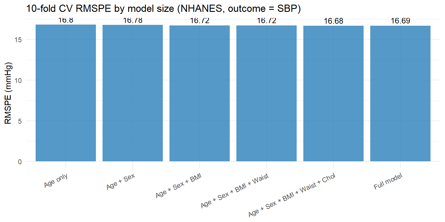
# Compare test RMSPE for models with 1–6 predictors (forward order)
set.seed(42)
k <- 10
folds <- sample(rep(1:k, length.out = nrow(nhanes_cc)))

predictor_sets <- list(
  "Age only"              = "SBP ~ Age",
  "Age + Sex"             = "SBP ~ Age + Sex",
  "Age + Sex + BMI"       = "SBP ~ Age + Sex + BMI",
  "Age + Sex + BMI + Waist" = "SBP ~ Age + Sex + BMI + Waist",
  "Age + Sex + BMI + Waist + Chol" = "SBP ~ Age + Sex + BMI + Waist + Cholesterol",
  "Full model"            = "SBP ~ Age + Sex + BMI + Waist + Cholesterol + factor(Diabetes) + factor(Smoker)"
)

cv_rmspe <- sapply(predictor_sets, function(fmla) {
  sqrt(mean(sapply(1:k, function(j) {
    tr <- nhanes_cc[folds != j, ]
    te <- nhanes_cc[folds == j, ]
    fit <- lm(as.formula(fmla), data = tr)
    mean((te$SBP - predict(fit, newdata = te))^2, na.rm = TRUE)
  })))
})

res <- data.frame(Model = factor(names(cv_rmspe), levels = names(cv_rmspe)),
                  RMSPE = cv_rmspe)

ggplot(res, aes(x = Model, y = RMSPE)) +
  geom_col(fill = "#2980b9", alpha = 0.8) +
  geom_text(aes(label = round(RMSPE, 2)), vjust = -0.4, size = 3.5) +
  labs(title = "10-fold CV RMSPE by model size (NHANES, outcome = SBP)",
       x = NULL, y = "RMSPE (mmHg)") +
  theme_minimal() +
  theme(axis.text.x = element_text(angle = 25, hjust = 1))

---

4 Guided Practice

R is loading in the background — exercises below will be interactive once ready.

TipHints

• Look at the AIC trace from step() — it shows which predictor was added at each step and the AIC change
• A RMSPE difference of <0.5 mmHg between models is probably not clinically meaningful
• The 1-SE rule: if the simpler model is within 1 SE of the best, prefer it

---

5 Retrieval Challenge

NoteFurther reading

James et al. (2021). An Introduction to Statistical Learning. — Chapter 6.1 (Subset selection)