U6 — UMAP: Uniform Manifold Approximation and Projection

1 Concept: t-SNE’s Faster, More Structured Sibling

1.1 What UMAP adds over t-SNE

UMAP (Uniform Manifold Approximation and Projection) is a nonlinear dimensionality reduction method with a similar goal to t-SNE: project high-dimensional data into 2D while preserving local structure. It differs in two important ways:

	t-SNE	UMAP
Mathematical basis	KL divergence between probability distributions	Topological data analysis (Riemannian geometry)
Global structure	Often distorted — cluster distances not reliable	Better preserved — relative distances between clusters are more meaningful
Speed	Slow on large datasets	Substantially faster
Reproducibility	Stochastic by default	Reproducible for fixed seed
New data	Cannot project new points	Can project new observations onto existing embedding

1.2 Key hyperparameters

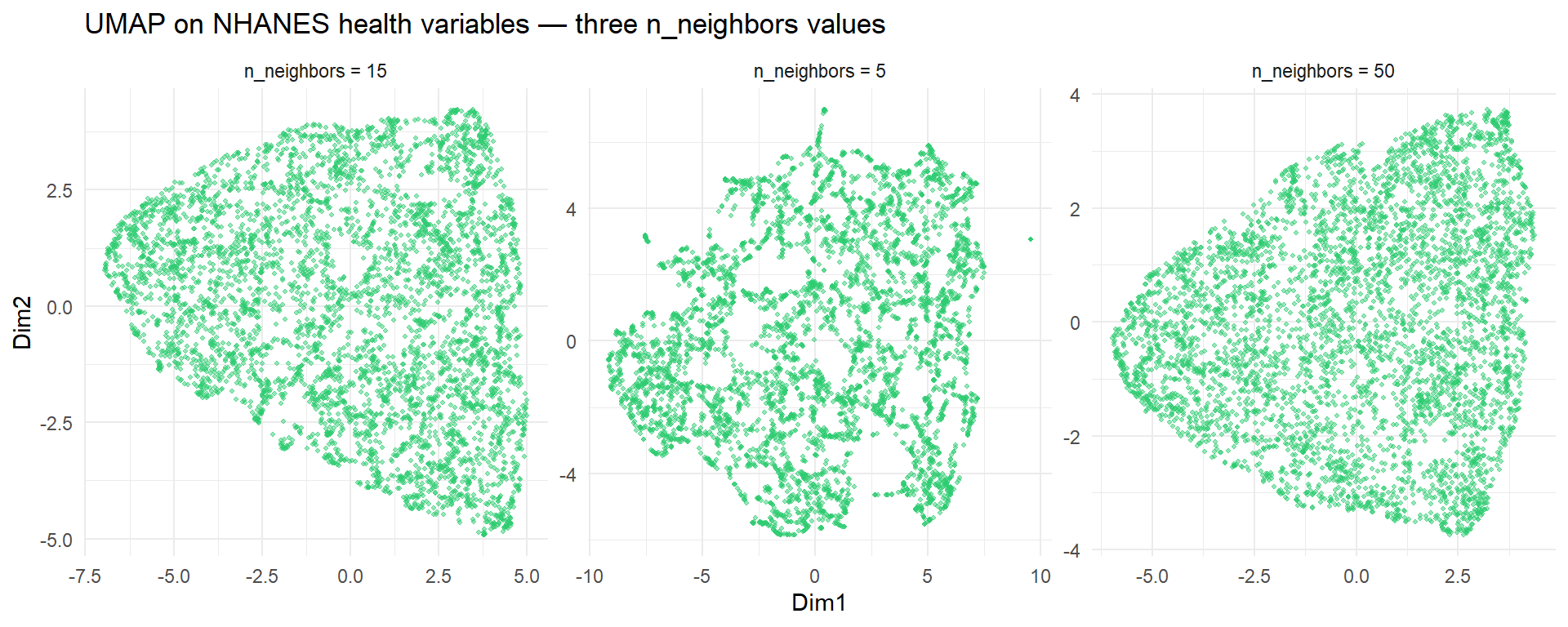
n_neighbors (default 15): How many neighbours each point considers. Like perplexity in t-SNE:

Low (e.g. 5): captures very local structure, can fragment real clusters
High (e.g. 50): captures broader structure, more similar to PCA

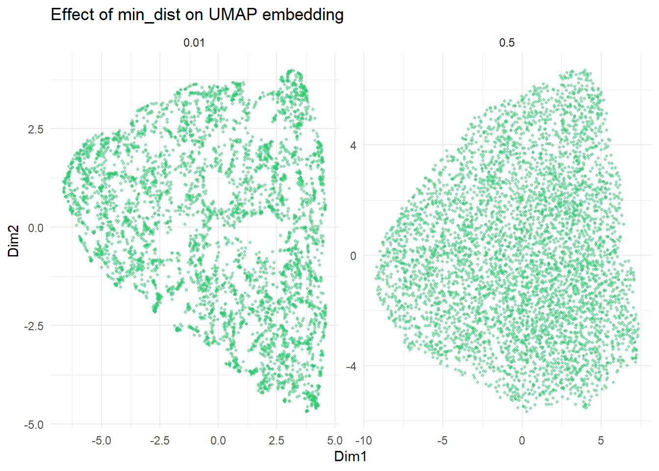
min_dist (default 0.1): How tightly points are packed in the 2D embedding:

Low (e.g. 0.01): tighter clusters, more separated
High (e.g. 0.5): smoother, more spread-out embedding

Run with multiple n_neighbors values to check stability, just as you would with t-SNE perplexity.

1.3 When to use UMAP vs t-SNE

For visualisation of high-dimensional data (scRNA-seq, image embeddings): both work; UMAP is now the default in most genomics pipelines
When global structure matters (are cluster A and cluster B more similar to each other than to cluster C?): prefer UMAP
When speed is a constraint on large datasets: prefer UMAP
For teaching and comparison: use both and compare

2 Quiz

Nothing — distances between clusters in UMAP are always completely arbitrary

A and C are more similar in the original space — UMAP preserves global distances better than t-SNE

Cluster B contains more observations and therefore occupies more visual space

This spatial layout is purely an artefact of the min_dist hyperparameter choice

UMAP's mathematical framework preserves global structure better than t-SNE: clusters that are genuinely more similar in the original space tend to appear closer in the UMAP embedding. This is not a strict guarantee, but it is more reliable than t-SNE, where cluster distances are largely meaningless. For t-SNE, the only reliable information is which points are near each other locally.

Increasing n_neighbors fragments the embedding into more, smaller disconnected clusters

More neighbours blur fine local structure and emphasise broader global patterns instead

The axes become interpretable as principal components once n_neighbors exceeds a certain threshold

The UMAP algorithm fails to converge and produces empty output when n_neighbors is set too high

n_neighbors controls the size of the local neighbourhood each point uses to build its representation of the manifold. Small n_neighbors captures fine-grained local structure but can fragment real clusters. Large n_neighbors considers more global context, producing smoother embeddings that resemble PCA more closely. The default of 15 is a reasonable starting point; always try at least one smaller and one larger value.

UMAP finds more clusters than t-SNE on any dataset due to its superior optimisation algorithm

UMAP needs no hyperparameter tuning — unlike t-SNE, all default settings produce reliable results

UMAP's computational efficiency makes it far more practical than t-SNE at 100k+ observations

UMAP axes are interpretable like PCA components, representing the main directions of variance in the data

t-SNE uses Barnes-Hut approximation to achieve O(n log n) complexity, which is still slow for hundreds of thousands of points. UMAP uses approximate nearest-neighbour graphs and stochastic gradient descent, scaling much better to large datasets. On PBMC3k (2638 cells), both are fast. On a full single-cell atlas with 500 000 cells, UMAP runs in minutes while t-SNE may take hours.

3 Worked Example: UMAP on NHANES Health Variables

vars <- c("Age", "BMI", "Waist", "Cholesterol", "SBP")
dat  <- na.omit(nhanes[, vars])
X    <- scale(dat)
set.seed(42)

# Three n_neighbors values
umap_5  <- umap(X, n_neighbors = 5,  min_dist = 0.1)
umap_15 <- umap(X, n_neighbors = 15, min_dist = 0.1)
umap_50 <- umap(X, n_neighbors = 50, min_dist = 0.1)

make_df <- function(res, nn) {
  data.frame(Dim1 = res[, 1], Dim2 = res[, 2],
             n_neighbors = paste("n_neighbors =", nn))
}

umap_all <- rbind(make_df(umap_5, 5),
                  make_df(umap_15, 15),
                  make_df(umap_50, 50))

ggplot(umap_all, aes(Dim1, Dim2)) +
  geom_point(size = 0.8, alpha = 0.5, colour = "#2ecc71") +
  facet_wrap(~ n_neighbors, scales = "free") +
  labs(title = "UMAP on NHANES health variables — three n_neighbors values") +
  theme_minimal()

library(Rtsne)
set.seed(42)
tsne30  <- Rtsne(X, dims = 2, perplexity = 30, check_duplicates = FALSE)

df_tsne <- data.frame(Dim1 = tsne30$Y[, 1], Dim2 = tsne30$Y[, 2],
                      Method = "t-SNE (perplexity = 30)", Age = dat$Age)
df_umap <- data.frame(Dim1 = umap_15[, 1],  Dim2 = umap_15[, 2],
                      Method = "UMAP (n_neighbors = 15)", Age = dat$Age)

ggplot(rbind(df_tsne, df_umap), aes(Dim1, Dim2, colour = Age)) +
  geom_point(size = 0.8, alpha = 0.6) +
  scale_colour_viridis_c(option = "plasma") +
  facet_wrap(~ Method, scales = "free") +
  labs(title = "t-SNE vs UMAP — coloured by Age") +
  theme_minimal()

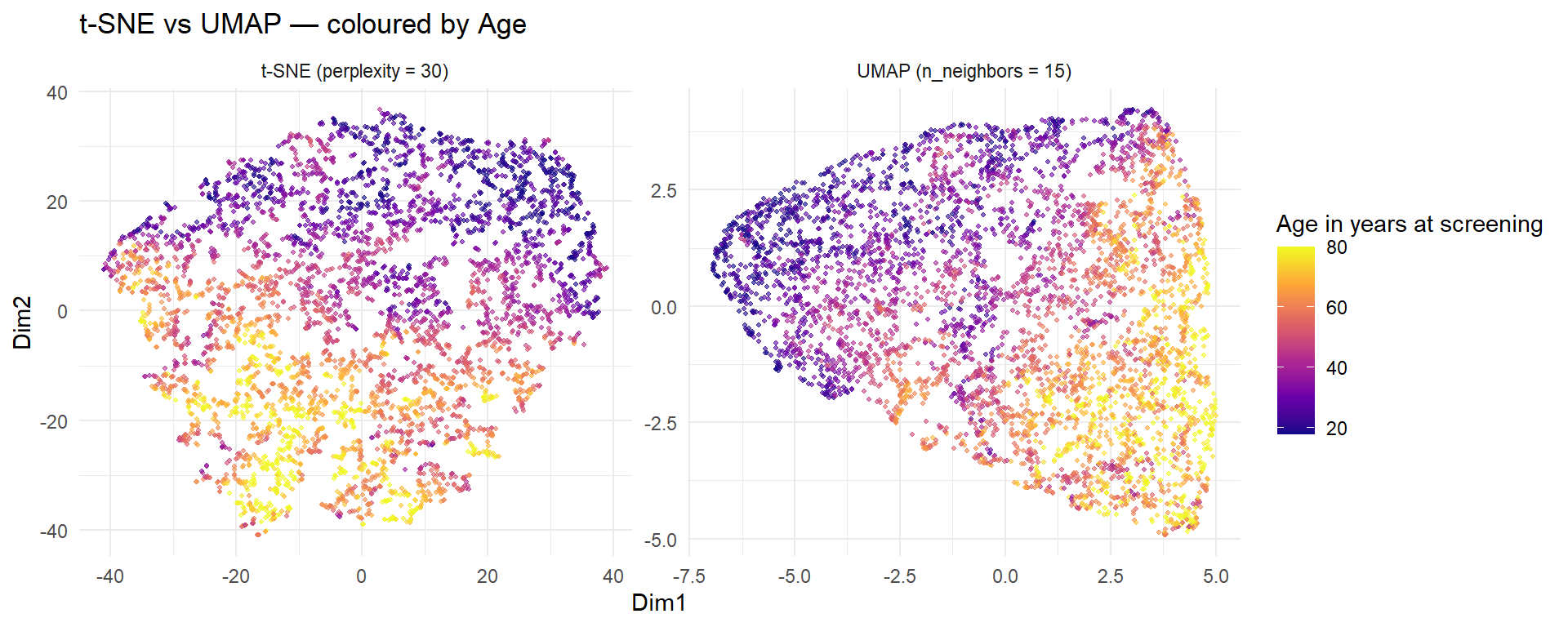
Interpretation: Both methods separate older and younger patients into visible gradients. With five variables, the difference is subtle. In Project 3 (PBMC3k scRNA-seq), UMAP and t-SNE separate 8+ cell types that are completely mixed in PCA space — this is where the methods show their real value.

4 Guided Practice

Note

Note: The uwot package requires compiled C++ dependencies that are not available in the browser-based R environment (WebR). The exercises below show pre-rendered output. Run the code in a local R session to interact with the results.

vars <- c("Age", "BMI", "Waist", "Cholesterol", "SBP")
dat  <- na.omit(nhanes[, vars])
X    <- scale(dat)
set.seed(42)

# TASK 1: Run UMAP with n_neighbors = 15, min_dist = 0.1
umap_res <- umap(X, n_neighbors = 15, min_dist = 0.1)

# TASK 2: Plot the result, coloured by SBP
df <- data.frame(Dim1 = umap_res[, 1], Dim2 = umap_res[, 2], SBP = dat$SBP)

ggplot(df, aes(Dim1, Dim2, colour = SBP)) +
  geom_point(size = 1, alpha = 0.6) +
  scale_colour_viridis_c() +
  labs(title = "UMAP — coloured by SBP") +
  theme_minimal()

vars <- c("Age", "BMI", "Waist", "Cholesterol", "SBP")
dat  <- na.omit(nhanes[, vars])
X    <- scale(dat)

# TASK 3: Compare min_dist = 0.01 vs min_dist = 0.5
# How does the compactness of the embedding change?
set.seed(42)
umap_tight  <- umap(X, n_neighbors = 15, min_dist = 0.01)
umap_spread <- umap(X, n_neighbors = 15, min_dist = 0.5)

df <- rbind(
  data.frame(Dim1 = umap_tight[, 1],  Dim2 = umap_tight[, 2],  min_dist = "0.01"),
  data.frame(Dim1 = umap_spread[, 1], Dim2 = umap_spread[, 2], min_dist = "0.5")
)

ggplot(df, aes(Dim1, Dim2)) +
  geom_point(size = 0.8, alpha = 0.5, colour = "#2ecc71") +
  facet_wrap(~ min_dist, scales = "free") +
  labs(title = "Effect of min_dist on UMAP embedding") +
  theme_minimal()

Hints

umap(X, n_neighbors = 15, min_dist = 0.1) returns an n×2 matrix
Index columns 1 and 2 for Dim1/Dim2
Low min_dist → points are pushed closer together → more compact clusters
High min_dist → points are spread out → smoother, more continuous embedding

5 Retrieval Challenge

# Full pipeline: scale → UMAP → K-means → visualise
# 1. Run UMAP with n_neighbors = 15 on the scaled NHANES data
# 2. Run k-means with K = 3 on the original scaled data (not UMAP coordinates)
# 3. Colour the UMAP plot by the K-means cluster assignment
# 4. Do the K-means clusters appear separated in UMAP space?

vars <- c("Age", "BMI", "Waist", "Cholesterol", "SBP")
dat  <- na.omit(nhanes[, vars])
X    <- scale(dat)
set.seed(42)

umap_res <- umap(X, n_neighbors = 15, min_dist = 0.1)
km3      <- kmeans(X, centers = 3, nstart = 25)

df <- data.frame(
  Dim1    = umap_res[, 1],
  Dim2    = umap_res[, 2],
  cluster = factor(km3$cluster)
)

ggplot(df, aes(Dim1, Dim2, colour = cluster)) +
  geom_point(size = 1, alpha = 0.6) +
  scale_colour_manual(values = c("#e74c3c", "#3498db", "#2ecc71")) +
  labs(title = "K-means clusters (K = 3) visualised in UMAP space") +
  theme_minimal()

Model Answer

umap_res <- umap(X, n_neighbors = 15, min_dist = 0.1)
km3      <- kmeans(X, centers = 3, nstart = 25)

df <- data.frame(
  Dim1    = umap_res[, 1],
  Dim2    = umap_res[, 2],
  cluster = factor(km3$cluster)
)

ggplot(df, aes(Dim1, Dim2, colour = cluster)) +
  geom_point(size = 1, alpha = 0.6) +
  scale_colour_manual(values = c("#e74c3c", "#3498db", "#2ecc71")) +
  labs(title = "K-means clusters (K = 3) visualised in UMAP space") +
  theme_minimal()

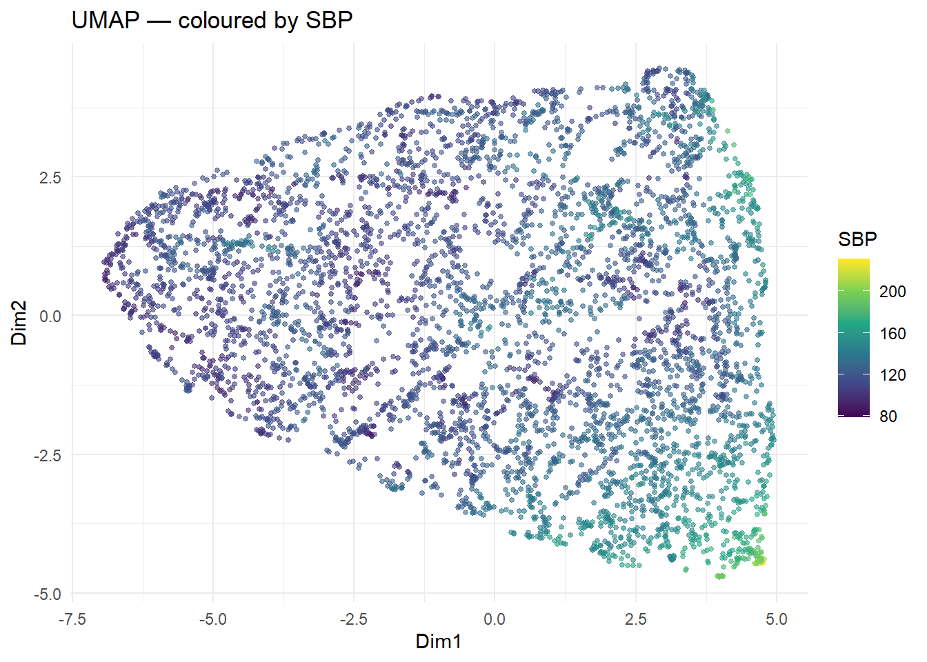
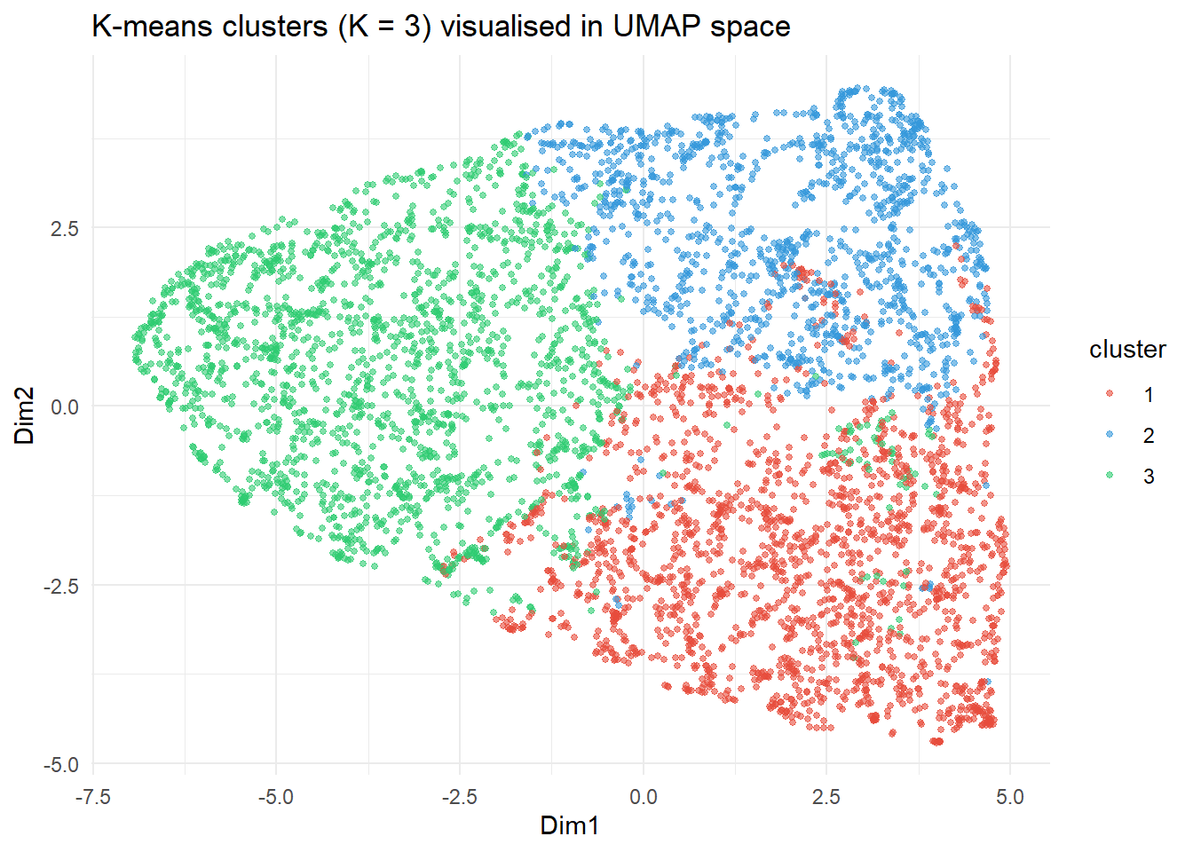
If the k-means clusters appear well-separated in the UMAP plot, it confirms that UMAP has captured the same structure. If they overlap, it suggests either the clusters are not well-separated in the original space, or UMAP and k-means are picking up different aspects of the data structure.

6 Why-Questions

Q: “For the PBMC3k scRNA-seq data in Project 3, should I use PCA, t-SNE, or UMAP?”

The standard pipeline is: (1) PCA on the 2000 variable genes to reduce to 20–50 PCs; (2) UMAP (or t-SNE) on the PC scores for 2D visualisation; (3) cluster in PCA space (Seurat uses a graph-based Louvain algorithm on the PC-space nearest-neighbour graph). UMAP is now the default in Seurat. PCA alone is not sufficient — the cell type structure is nonlinear and only visible after UMAP/t-SNE.

Q: “If I run UMAP twice with the same seed, do I get the same result?”

Yes — unlike t-SNE, UMAP is reproducible for a fixed seed. This makes it preferable for published figures and for comparing results across analyses. Set set.seed() immediately before calling umap(). Note that the result will still change if you change any hyperparameter (n_neighbors, min_dist) or if the data changes.

Q: “Do the axes of a UMAP plot have any meaning?”

No — like t-SNE, the axes have no intrinsic meaning. UMAP1 is not the direction of maximum variance (that is PC1). The axes can be rotated, reflected, or scaled without changing the information content. What matters is the relative position of points: nearby points were similar in the original high-dimensional space. When publishing or reporting UMAP plots, label the axes “UMAP1” and “UMAP2” and always state the n_neighbors and min_dist values used.