U4 — PAM: Partitioning Around Medoids

1 Concept: A More Robust Alternative to K-Means

1.1 Medoids vs centroids

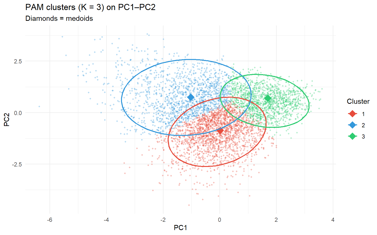
K-means represents each cluster by its centroid — the mean of all observations in that cluster. The centroid is usually not an actual data point. PAM uses a medoid instead: the actual observation that minimises the total dissimilarity to all other members of its cluster.

	K-means	PAM
Cluster representative	Centroid (mean — not a real data point)	Medoid (an actual observation)
Objective	Minimise total within-cluster SS	Minimise total dissimilarity to medoids
Robustness to outliers	Low — mean shifts toward extremes	Higher — medoid is a typical, central point
Must choose K?	Yes	Yes
Distance measure	Euclidean only	Any dissimilarity matrix

Because the medoid is an actual observation, PAM clusters are more interpretable: you can inspect the representative patient directly rather than a hypothetical average.

1.2 The silhouette width

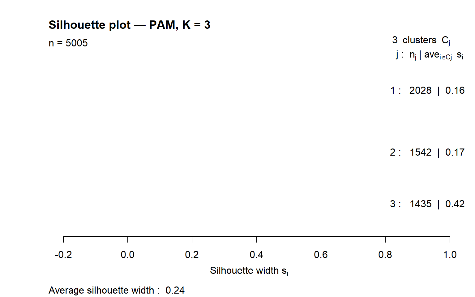
PAM uses the silhouette width as a built-in quality measure. For each observation $i$:

\[s(i) = \frac{b(i) - a(i)}{\max(a(i),\, b(i))}\]

where $a(i)$ is the mean distance to other observations in the same cluster, and $b(i)$ is the mean distance to observations in the nearest other cluster.

Value	Interpretation
$s(i) \approx 1$	Observation fits well inside its cluster
$s(i) \approx 0$	Observation lies on the border between two clusters
$s(i) < 0$	Observation may belong to a neighbouring cluster

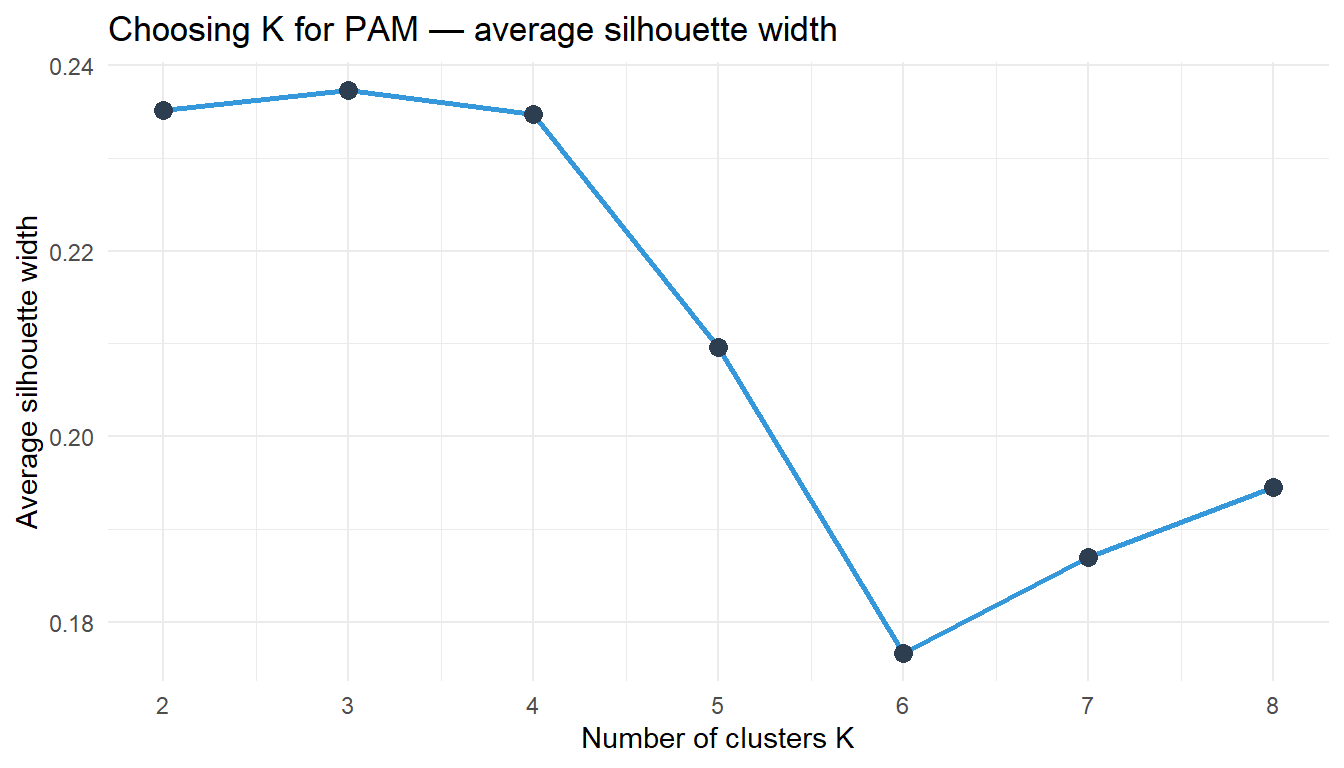
The average silhouette width summarises overall cluster quality. To choose K, run PAM for K = 2, 3, … and pick the K that maximises the average silhouette width.

1.3 Scaling

PAM uses dissimilarities (Euclidean by default). Like k-means, standardise all variables before running PAM so no single variable dominates the distance calculation.

2 Quiz

A medoid is the mean of the cluster — identical to a K-means centroid

The cluster member minimising total dissimilarity to all others — always an actual observation, not a computed mean

A medoid is the observation with the largest distance to the cluster centre

A medoid is a concept exclusive to hierarchical clustering, not used in PAM

The centroid is the mean vector — it represents the "average" observation and is usually not one of the actual data points. The medoid is an actual observation that is most central. For clinical interpretation, the medoid is more useful: you can look up patient 42 and read their actual record, rather than a hypothetical mean patient with Age = 54.3 and BMI = 27.1.

The patient is well-assigned — a negative silhouette indicates strong cluster membership

The patient sits exactly on the boundary between two equally close clusters

This patient is closer on average to a neighbouring cluster than to their own — likely misassigned

The clustering algorithm failed to converge on a stable assignment for this patient

A negative silhouette means b(i) < a(i): the observation is on average closer to members of another cluster than to its own. This suggests the observation is in the wrong cluster, or that the clusters are not well-separated at this value of K. It does not mean the algorithm failed — it just means this particular observation sits in an ambiguous region of the data.

K = 2, because simpler is always better

K = 3, because it has the highest average silhouette width

K = 5, because more clusters capture more variation

None — a maximum silhouette of 0.44 is too low to trust

The silhouette method selects the K that maximises the average silhouette width. K = 3 gives 0.44, the highest value, so it provides the best separation given the data geometry. There is no absolute threshold for "good enough" silhouette — 0.44 indicates reasonable but not perfect structure. Compare to an elbow plot from k-means to see if both methods agree.

3 Worked Example: Patient Profiles with PAM in NHANES

vars <- c("Age", "BMI", "Waist", "Cholesterol", "SBP")
dat  <- na.omit(nhanes[, vars])
X    <- scale(dat)

# Choose K using average silhouette width
set.seed(42)
sil_widths <- sapply(2:8, function(k) pam(X, k = k)$silinfo$avg.width)
data.frame(K = 2:8, AvgSilhouette = round(sil_widths, 3))

  K AvgSilhouette
1 2         0.235
2 3         0.237
3 4         0.235
4 5         0.210
5 6         0.177
6 7         0.187
7 8         0.195

ggplot(data.frame(K = 2:8, sil = sil_widths), aes(K, sil)) +
  geom_line(colour = "#3498db", linewidth = 1) +
  geom_point(size = 3, colour = "#2c3e50") +
  scale_x_continuous(breaks = 2:8) +
  labs(title = "Choosing K for PAM — average silhouette width",
       x = "Number of clusters K", y = "Average silhouette width") +
  theme_minimal()

set.seed(42)
pam3 <- pam(X, k = 3)

# The medoids — actual row numbers in X
pam3$id.med

[1] 4889  411  563

# Medoid profiles on original scale
dat[pam3$id.med, ]

# A tibble: 3 × 5
    Age   BMI Waist Cholesterol   SBP
  <dbl> <dbl> <dbl>       <dbl> <dbl>
1    59  26.9  95.7         200  131.
2    46  34.7 117           182  123.
3    28  24.2  84.5         165  111.

plot(silhouette(pam3), main = "Silhouette plot — PAM, K = 3")

pca <- prcomp(X)
scores <- data.frame(pca$x[, 1:2], cluster = factor(pam3$clustering))
medoid_scores <- scores[pam3$id.med, ]

ggplot(scores, aes(PC1, PC2, colour = cluster)) +
  geom_point(alpha = 0.3, size = 0.8) +
  geom_point(data = medoid_scores, size = 5, shape = 18) +
  stat_ellipse(linewidth = 0.8) +
  scale_colour_manual(values = c("#e74c3c", "#3498db", "#2ecc71")) +
  labs(title = "PAM clusters (K = 3) on PC1–PC2",
       subtitle = "Diamonds = medoids",
       colour = "Cluster") +
  theme_minimal()

Interpretation: The medoids are real patients — you can read their actual Age, BMI, SBP, etc. This is a key interpretive advantage over k-means, where the centroid is a hypothetical average.

4 Guided Practice

R is loading in the background — exercises will be interactive once the status bar disappears.

Hints

pam(X, k = K)$silinfo$avg.width returns the average silhouette for K clusters
pam3$id.med gives the row indices of the medoids in X
Index into dat (unscaled) to read medoid profiles in interpretable units
Compare the silhouette plot to the k-means elbow — do they agree on K?

5 Retrieval Challenge

Model Answer

pam3 <- pam(X, k = 3)
km3  <- kmeans(X, centers = 3, nstart = 25)

# Cross-tabulation — rows = PAM, columns = K-means
table(PAM = pam3$clustering, KMeans = km3$cluster)

# Note: cluster labels are arbitrary — the same cluster may be
# labelled "1" in PAM and "2" in K-means

The cross-table typically shows high agreement — most cells in each row have one dominant column. Where they disagree is often near cluster boundaries, where the medoid-based and centroid-based rules pull in different directions.

6 Why-Questions

Q: “When should I use PAM instead of K-means?”

Use PAM when: (1) interpretability matters and you want a real representative patient, not a hypothetical average; (2) the data contain outliers that could shift a K-means centroid; (3) you want a built-in quality measure (silhouette) to guide the choice of K. K-means is preferred when n is very large (PAM is O(n²) per iteration, k-means is O(nKd)) or when you need fast re-clustering of new observations.

Q: “A silhouette of 0.3 — is that good or bad?”

Silhouette values above 0.5 are generally considered strong structure; 0.25–0.5 is weak but present; below 0.25 suggests no real cluster structure. However, these thresholds depend on the number of dimensions and the nature of the data. Health data with many correlated variables often produces moderate silhouettes even when the clusters are clinically meaningful. Always combine silhouette width with clinical interpretation of the cluster profiles.

Q: “How does PAM connect to what I did in the STA230 exercises?”

In Exercise 5, you ran PAM on the iris dataset and used the silhouette plot to evaluate whether K = 2 or K = 3 best described the flower measurements. You saw that setosa was well-separated (high silhouette) while versicolor and virginica overlapped (lower silhouette). The same logic applies here: NHANES patients in the “healthy” profile cluster tightly, while borderline patients near the cluster boundary have lower silhouette values.