R5 — Model Comparison & Workflow

1 Concept: Putting It All Together

1.1 The complete regression workflow

1. Explore data          → distributions, missingness, outliers
2. Pre-process           → log-transform skewed outcomes, standardise predictors
3. Split data            → train (70%) / test (30%) — or use CV throughout
4. Fit candidate models  → OLS, forward stepwise, ridge, LASSO
5. Select model          → by CV RMSPE on training data only
6. Evaluate              → test RMSPE on held-out test set (once, at the end)
7. Report                → coefficients, CIs, test performance, clinical interpretation

The golden rule

The test set is used exactly once — at the end. If you look at the test set to make model choices, it is no longer a clean test set.

1.2 Which method to choose?

Situation	Recommended method
\(p\) small, inference goal	OLS with stepwise/AIC selection
\(p\) moderate, prediction goal	LASSO or elastic net
\(p\) large, many small effects	Ridge
Correlated predictors	Ridge or elastic net
Need sparse, interpretable model	LASSO

1.3 Reporting test performance

Report RMSPE (or MAE) on the test set with a confidence interval:

\[\text{RMSPE} \pm 1.96 \times \frac{\text{SD of squared errors}}{\sqrt{n_{\text{test}}}}\]

Never report only training performance. Always compare to a baseline (e.g., predicting the mean: \(\text{RMSPE}_{\text{null}} = \text{SD}(Y)\)).

2 Quiz

Nothing — comparing methods on the test set is the correct approach

Selecting the best model using the test set makes the reported RMSPE optimistically biased

You cannot compare different model classes on the same test set

The test RMSPE is only valid if all models use the same lambda

If you pick the model with the lowest test RMSPE, the reported performance is optimistic — you effectively selected the model that happened to fit the test data best. This is a subtle form of overfitting. The fix: use cross-validation on training data for model selection, then report performance on a truly held-out test set that was never used during model building.

LASSO is excellent — any improvement over the null confirms strong clinical value

The model is useless since it doesn't approach perfect prediction

An ~11% reduction over the null is modest — clinical relevance requires domain interpretation

The null model is an inappropriate baseline — only absolute RMSPE values are meaningful

The null RMSPE (SD of Y) is the natural baseline — it's what you get by ignoring all predictors. Going from 18 to 16 mmHg (~11% reduction) is a meaningful but modest improvement. Whether it's clinically useful depends on the application. For individual patient risk prediction, 16 mmHg error may still be too imprecise. Always contextualise RMSPE against domain-specific requirements.

3 Worked Example: Full Comparison on NHANES

set.seed(42)
tr_idx <- sample(nrow(nhanes_cc), round(0.7 * nrow(nhanes_cc)))
X_tr <- X[tr_idx, ];  y_tr <- y[tr_idx]
X_te <- X[-tr_idx, ]; y_te <- y[-tr_idx]

# Null model baseline
null_rmspe <- sqrt(mean((y_te - mean(y_tr))^2))

# OLS
ols <- lm(y_tr ~ X_tr)
ols_rmspe <- sqrt(mean((y_te - cbind(1, X_te) %*% coef(ols))^2))

# Forward stepwise (AIC) — refit on training data
tr_df <- as.data.frame(cbind(SBP = y_tr, X_tr))
fwd <- step(lm(SBP ~ 1, data=tr_df),
            scope = list(upper = lm(SBP ~ ., data=tr_df)),
            direction = "forward", trace = FALSE)
te_df <- as.data.frame(cbind(SBP = y_te, X_te))
fwd_rmspe <- sqrt(mean((y_te - predict(fwd, newdata=te_df))^2))

# Ridge and LASSO via CV
cv_ridge <- cv.glmnet(X_tr, y_tr, alpha = 0, nfolds = 10)
cv_lasso <- cv.glmnet(X_tr, y_tr, alpha = 1, nfolds = 10)
ridge_rmspe <- sqrt(mean((y_te - predict(cv_ridge, X_te, s="lambda.min"))^2))
lasso_rmspe <- sqrt(mean((y_te - predict(cv_lasso, X_te, s="lambda.min"))^2))

# Summary table
results <- data.frame(
  Method = c("Null (mean)", "OLS", "Forward (AIC)", "Ridge", "LASSO"),
  Test_RMSPE = round(c(null_rmspe, ols_rmspe, fwd_rmspe, ridge_rmspe, lasso_rmspe), 3)
)
results$vs_Null <- round(100 * (1 - results$Test_RMSPE / null_rmspe), 1)
names(results)[3] <- "% better than null"
print(results)

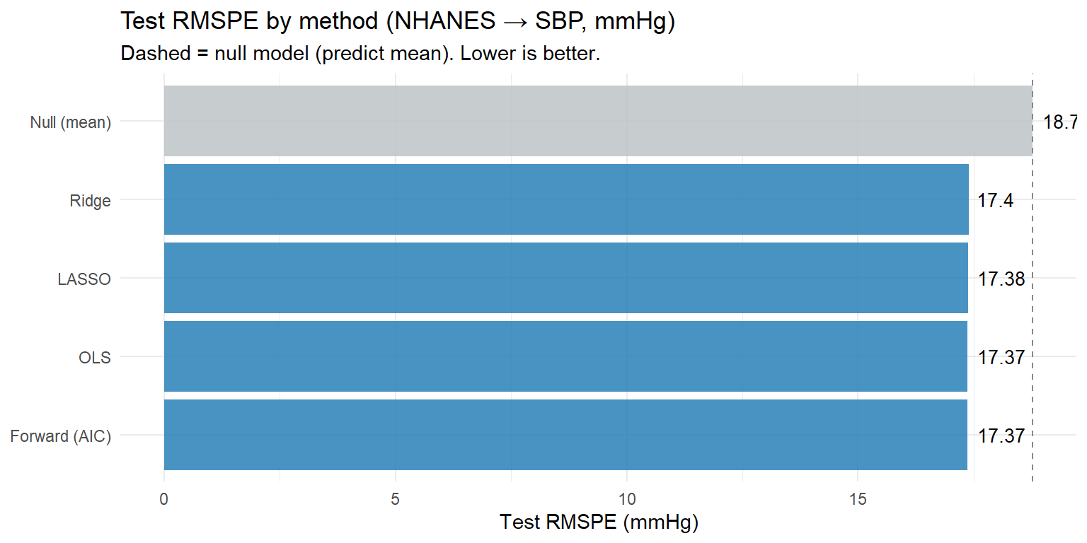
         Method Test_RMSPE % better than null
1   Null (mean)     18.777                0.0
2           OLS     17.368                7.5
3 Forward (AIC)     17.368                7.5
4         Ridge     17.398                7.3
5         LASSO     17.375                7.5

ggplot(results, aes(x = reorder(Method, Test_RMSPE),
                     y = Test_RMSPE, fill = Method == "Null (mean)")) +
  geom_col(alpha = 0.85) +
  geom_hline(yintercept = null_rmspe, linetype = "dashed", colour = "#888") +
  geom_text(aes(label = round(Test_RMSPE, 2)), hjust = -0.2, size = 3.5) +
  coord_flip() +
  scale_fill_manual(values = c("TRUE" = "#bdc3c7", "FALSE" = "#2980b9"),
                    guide = "none") +
  labs(title = "Test RMSPE by method (NHANES → SBP, mmHg)",
       subtitle = "Dashed = null model (predict mean). Lower is better.",
       x = NULL, y = "Test RMSPE (mmHg)") +
  theme_minimal()

4 Guided Practice: Full Workflow

R is loading in the background — exercises below will be interactive once ready.

Questions to answer

Does regularisation (ridge or LASSO) outperform plain OLS on this dataset? Why or why not?
Which predictors does LASSO select? Are they clinically plausible?
How much better is the best model vs the null baseline (in % RMSPE reduction)?
Is an RMSPE of ~16 mmHg clinically useful for individual SBP prediction?

5 Why-Questions

Q: “Should I report OLS p-values after doing LASSO selection?”

No — this is selective inference, and p-values are invalid after model selection. LASSO selected the variables partly based on the data, so performing OLS inference on the selected subset gives inflated Type I error. Options: (1) report only prediction performance from LASSO; (2) use a pre-specified confirmatory model for inference; (3) use methods designed for post-selection inference (e.g., the selectiveInference package).

Q: “My train and test RMSPE are nearly identical. Is that good?”

It means the model generalises well — no overfitting. With n=3500 training and p=7, OLS already has low variance, so regularisation adds little. Large train-test gaps indicate overfitting; nearly equal performance indicates good generalisation.