R4 — LASSO

1 Concept: Regularisation via L1 Penalty

1.1 The LASSO objective

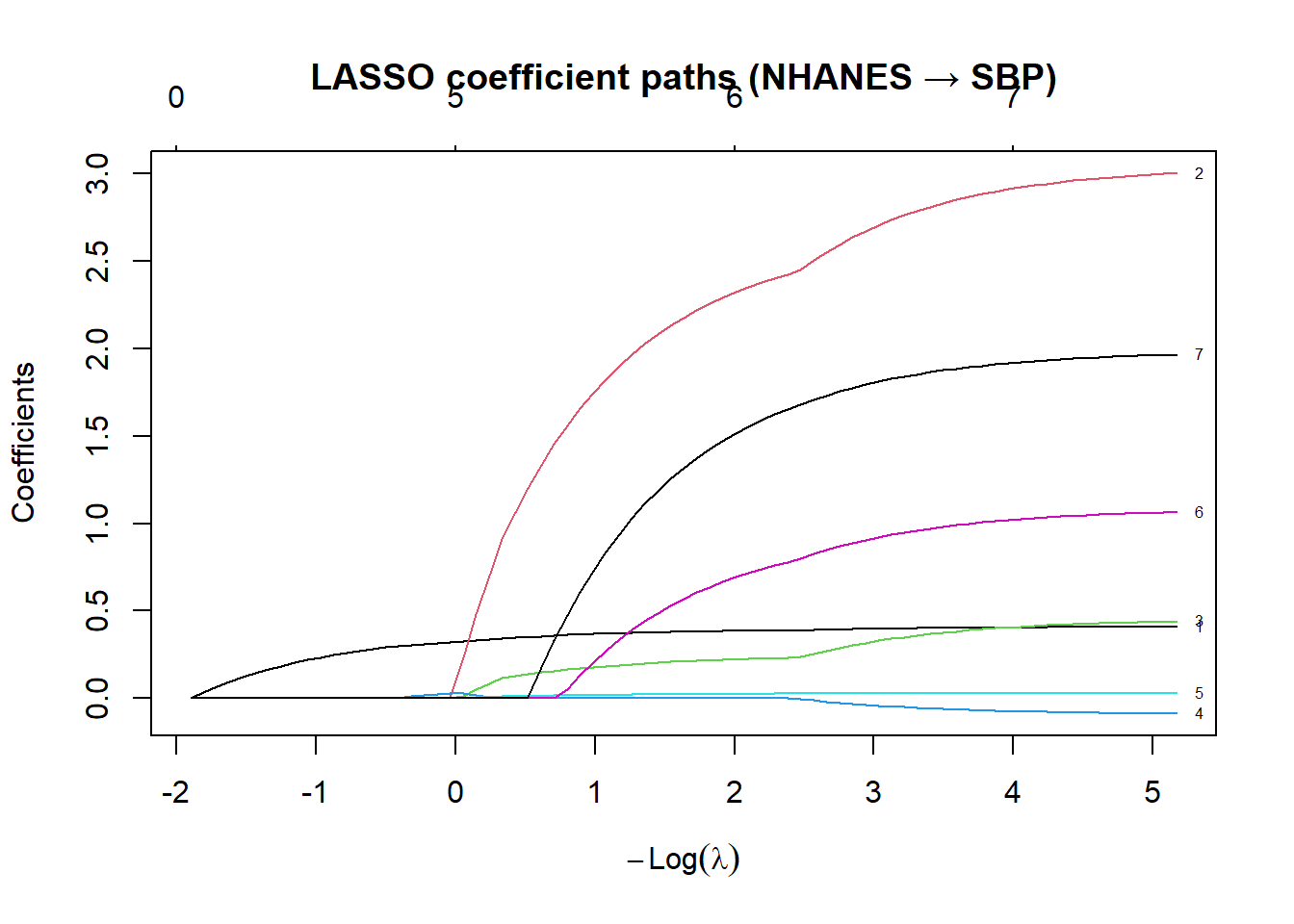
LASSO (Least Absolute Shrinkage and Selection Operator) uses an \(L_1\) penalty:

\[\hat{\boldsymbol{\beta}}^{\text{lasso}} = \arg\min_{\boldsymbol{\beta}} \left\{ \sum_{i=1}^n (y_i - \mathbf{x}_i^\top\boldsymbol{\beta})^2 + \lambda \sum_{j=1}^p |\beta_j| \right\}\]

The key difference from ridge: the \(L_1\) penalty produces sparse solutions — many \(\hat{\beta}_j = 0\) exactly. LASSO does variable selection automatically.

1.2 Why does L1 produce zeros?

Geometrically, the \(L_1\) constraint region (a diamond in 2D) has corners on the axes. The OLS ellipsoidal contours are likely to first touch one of these corners, where one or more \(\beta_j = 0\). The \(L_2\) constraint (a circle) has no corners, so the solution is rarely exactly zero.

1.3 LASSO vs Ridge

	LASSO	Ridge
Penalty	\(\lambda \sum \|\beta_j\|\)	\(\lambda \sum \beta_j^2\)
Sparsity	Yes — sets coefficients to exactly 0	No — shrinks toward 0 but not to 0
Variable selection	Yes	No
Best when	Few predictors truly matter	Many predictors with small effects
Correlated predictors	Selects one arbitrarily	Shrinks all equally

1.4 Elastic Net

The elastic net combines both penalties:

\[\lambda \left[\alpha \sum |\beta_j| + (1-\alpha) \sum \beta_j^2 \right]\]

With \(\alpha=1\) this is LASSO; \(\alpha=0\) is ridge. Elastic net handles correlated predictors better than pure LASSO. In glmnet(), alpha controls the mix.

2 Quiz

It always produces a lower test MSE than ridge

It performs automatic variable selection — only predictors with non-zero coefficients remain

It avoids the need for cross-validation to choose λ

It guarantees unbiased coefficient estimates for non-zero predictors

LASSO's sparsity is its key practical advantage. When p is large (say 100 predictors), LASSO might select 8 non-zero coefficients — these form a concise, interpretable model. In biostatistics, this is often exactly what's needed: a clinical risk score with a small number of measurable variables. Note: LASSO coefficients are biased (shrunk toward zero), so they should not be used directly for inference without correction.

lambda.min — it minimises CV error so it is always the best choice

lambda.1se — the sparsest model whose CV error is within 1 SE of the minimum, favouring parsimony

lambda.min for prediction, lambda.1se for hypothesis testing

lambda.1se — it always has lower test MSE

lambda.min gives the best average CV performance. lambda.1se uses the 1-SE rule: pick the largest λ (most regularisation, fewest non-zero predictors) whose CV error is within 1 standard error of the minimum. Since the CV errors are often not statistically different across a range of λ, the 1-SE model is sparser but statistically comparable — a good default for building parsimonious models.

Includes both with equal coefficients

Excludes both since they are redundant

Arbitrarily keeps one and zeroes the other — no unique solution exists when r=1

Crashes — LASSO cannot handle perfectly correlated predictors

With perfect correlation, the LASSO problem has many equivalent solutions (any split of the effect between X1 and X2 gives the same fit). LASSO arbitrarily picks one. Elastic net handles this better: it groups correlated predictors and shrinks them together, distributing the effect across the group. For highly correlated predictors (like BMI and waist circumference), elastic net is more stable than LASSO.

3 Worked Example

lasso_fit <- glmnet(X, y, alpha = 1)
plot(lasso_fit, xvar = "lambda", label = TRUE,
     main = "LASSO coefficient paths (NHANES → SBP)")

set.seed(42)
cv_lasso <- cv.glmnet(X, y, alpha = 1, nfolds = 10)
plot(cv_lasso)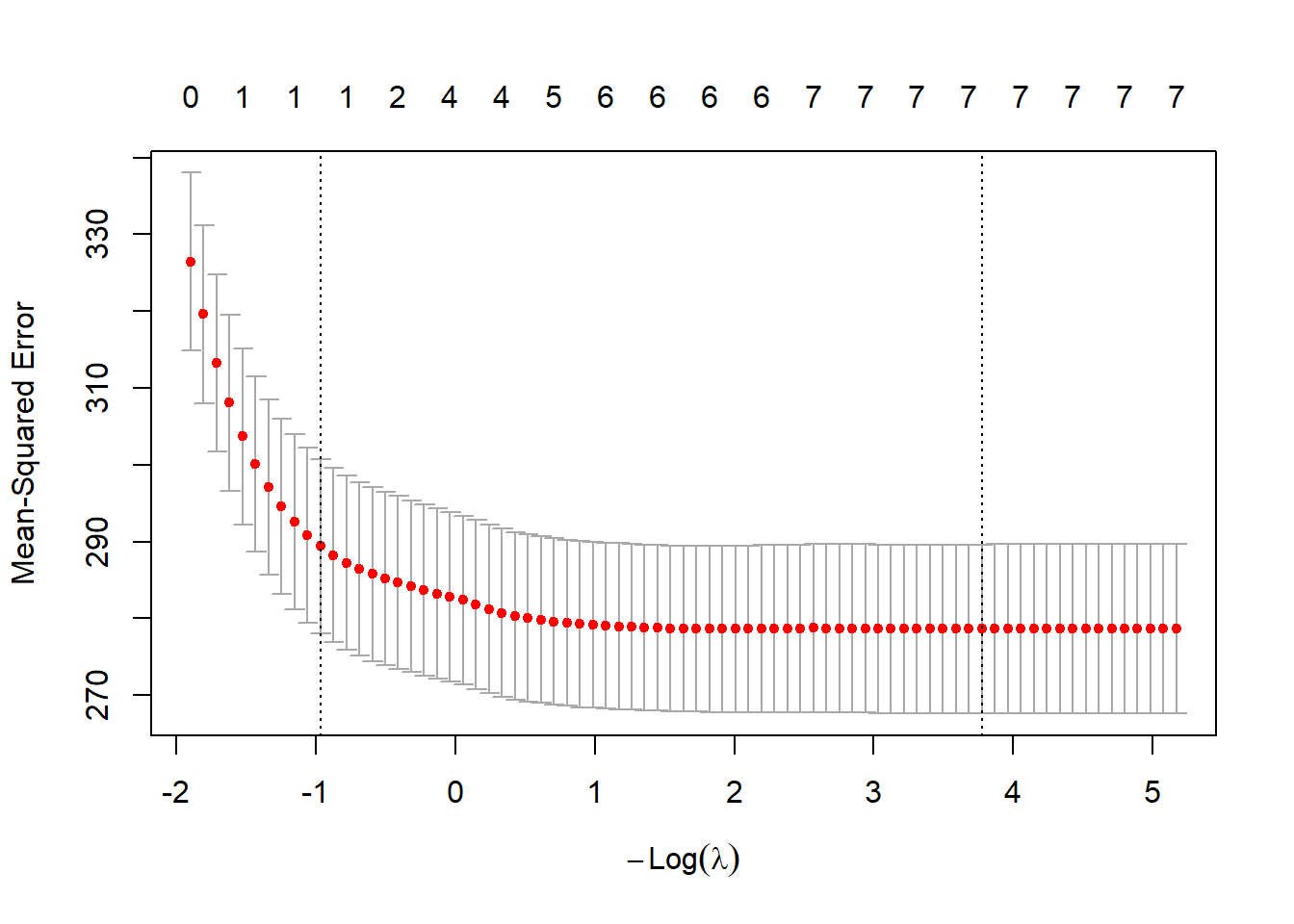

cat("lambda.min:", round(cv_lasso$lambda.min, 4), "\n")

lambda.min: 0.0229

cat("lambda.1se:", round(cv_lasso$lambda.1se, 4), "\n")

lambda.1se: 2.6356

# Coefficients at lambda.1se
coef_1se <- coef(cv_lasso, s = "lambda.1se")
cat("\nNon-zero coefficients at lambda.1se:\n")


Non-zero coefficients at lambda.1se:

nonzero <- coef_1se[coef_1se[, 1] != 0, , drop = FALSE]
print(round(nonzero, 4))

2 x 1 sparse Matrix of class "dgCMatrix"
            lambda.1se
(Intercept)   114.7632
Age             0.2344

cat("\nNumber of non-zero predictors:", nrow(nonzero) - 1, "\n")


Number of non-zero predictors: 1

# Compare LASSO, Ridge, and OLS on train/test
set.seed(42)
tr_idx <- sample(nrow(nhanes_cc), round(0.7 * nrow(nhanes_cc)))
X_tr <- X[tr_idx, ];  y_tr <- y[tr_idx]
X_te <- X[-tr_idx, ]; y_te <- y[-tr_idx]

cv_l <- cv.glmnet(X_tr, y_tr, alpha = 1, nfolds = 10)
cv_r <- cv.glmnet(X_tr, y_tr, alpha = 0, nfolds = 10)
ols  <- lm(y_tr ~ X_tr)

rmspe <- function(pred, ytrue) sqrt(mean((ytrue - pred)^2))

cat("OLS test RMSPE:   ", round(rmspe(cbind(1, X_te) %*% coef(ols), y_te), 3), "\n")

OLS test RMSPE:    17.368

cat("Ridge test RMSPE: ", round(rmspe(predict(cv_r, X_te, s="lambda.min"), y_te), 3), "\n")

Ridge test RMSPE:  17.398

cat("LASSO test RMSPE: ", round(rmspe(predict(cv_l, X_te, s="lambda.min"), y_te), 3), "\n")

LASSO test RMSPE:  17.373

4 Guided Practice

R is loading in the background — exercises below will be interactive once ready.

What to compare

Does LASSO zero out BMI or Waist? They are correlated — LASSO may arbitrarily pick one
Does elastic net handle this differently?
Is the test RMSPE meaningfully different between methods?

5 Retrieval Challenge

Model answer

With n=200 and p=20, LASSO should recover X2, X5, X11 reasonably well. lambda.1se tends to be more conservative (fewer predictors) and may miss weak signals (X11 with β=1.5). lambda.min includes more predictors and is more likely to recover all three but may also include false positives.