U5 — t-SNE: Nonlinear Dimensionality Reduction

1 Concept: Seeing Structure That PCA Misses

1.1 PCA is linear — that is a limitation

PCA finds the directions of maximum variance by a linear transformation of the data. If the true structure is curved or folded — as is common in high-dimensional biological or image data — PCA flattens it out and loses the local neighbourhood relationships.

t-SNE (t-distributed Stochastic Neighbour Embedding) is a nonlinear method designed to preserve local structure: observations that are close in high-dimensional space are placed close together in the 2D map.

1.2 How t-SNE works (intuitively)

In the high-dimensional space, compute a probability that observation $j$ is a neighbour of $i$: observations close together get high probability, distant ones near zero.
In the 2D embedding, compute corresponding probabilities.
Minimise the KL divergence between the two probability distributions by adjusting the 2D positions.

The result is a 2D map that reflects the local neighbourhood structure. Unlike PCA, the axes of a t-SNE plot have no interpretation — they are not “components” explaining variance. The distances between clusters are also not directly interpretable.

1.3 Perplexity

Perplexity is the main hyperparameter. It controls how many neighbours each observation “cares about” when building the high-dimensional probability distribution.

Perplexity	Effect
Low (e.g. 5)	Focuses on very local structure — can fragment real clusters
Medium (e.g. 30)	Standard default — balances local and semi-global structure
High (e.g. 100)	Considers more neighbours — blurs local detail, shows broader structure

Always run t-SNE with multiple perplexity values and check whether the structure is stable.

1.4 Important limitations

t-SNE is stochastic — different runs give different layouts. Use set.seed().
Cluster sizes and distances in the 2D plot are not meaningful — a compact cluster is not necessarily more homogeneous than a spread-out one.
t-SNE is designed for high-dimensional data (hundreds or thousands of variables). On five NHANES variables it is demonstrative only; PCA is usually sufficient at low dimensions.
t-SNE does not produce a transformation that can be applied to new data (unlike PCA).

2 Quiz

t-SNE maximises explained variance globally; PCA preserves local neighbourhood proximity in the 2D map

PCA captures global linear variance; t-SNE embeds data to preserve local neighbourhood structure

They produce identical 2D projections — t-SNE is simply a computationally faster implementation of PCA

PCA applies to any numeric data; t-SNE is designed exclusively for high-dimensional image datasets

PCA rotates the data so the first two axes capture the most variance globally. Two observations that are close in PC1–PC2 space may actually be separated on a higher PC. t-SNE, by contrast, directly optimises 2D positions to reflect proximity in the full high-dimensional space. t-SNE often reveals cluster structure invisible to PCA, but the axes are meaningless and cluster distances cannot be compared.

Perplexity = 5, because more detail is always better

Perplexity = 50, because larger perplexity is always better

Neither — only structure stable across several perplexity values should be trusted

The average visual impression from combining the two plots

Very low perplexity makes t-SNE focus on tiny local neighbourhoods and can fragment real clusters into many small islands. Very high perplexity approaches PCA-like global structure and may merge distinct groups. Reliable structure appears consistently across a range of perplexity values (e.g. 15, 30, 100). If a cluster only appears at one perplexity, treat it with scepticism.

Yes — compact clusters in t-SNE always indicate high internal similarity

No — the size and shape of clusters in t-SNE plots are not directly interpretable

Yes, but only if perplexity > 30

Yes — this is the main advantage of t-SNE over PCA

t-SNE distorts distances to pack the high-dimensional structure into 2D. The algorithm can make a dense cluster look spread out and a loose cloud look compact, depending on the local neighbourhood sizes. Never interpret the physical size of clusters in a t-SNE plot as a measure of homogeneity. Use silhouette widths or within-cluster distances in the original space for that.

3 Worked Example: t-SNE on NHANES Health Variables

We use five health variables — note that t-SNE is most powerful for data with hundreds of variables. This example is illustrative; for scRNA-seq or image data the advantage over PCA is much larger.

vars <- c("Age", "BMI", "Waist", "Cholesterol", "SBP")
dat  <- na.omit(nhanes[, vars])
X    <- scale(dat)
set.seed(42)

# Run t-SNE with three perplexity values
tsne_15  <- Rtsne(X, dims = 2, perplexity = 15,  check_duplicates = FALSE)
tsne_30  <- Rtsne(X, dims = 2, perplexity = 30,  check_duplicates = FALSE)
tsne_100 <- Rtsne(X, dims = 2, perplexity = 100, check_duplicates = FALSE)

make_df <- function(res, perp) {
  data.frame(Dim1 = res$Y[, 1], Dim2 = res$Y[, 2],
             Perplexity = paste("Perplexity =", perp))
}

tsne_all <- rbind(make_df(tsne_15, 15),
                  make_df(tsne_30, 30),
                  make_df(tsne_100, 100))

ggplot(tsne_all, aes(Dim1, Dim2)) +
  geom_point(size = 0.8, alpha = 0.5, colour = "#3498db") +
  facet_wrap(~ Perplexity, scales = "free") +
  labs(title = "t-SNE on NHANES health variables — three perplexity values",
       subtitle = "Axes have no interpretation — only relative proximity matters") +
  theme_minimal()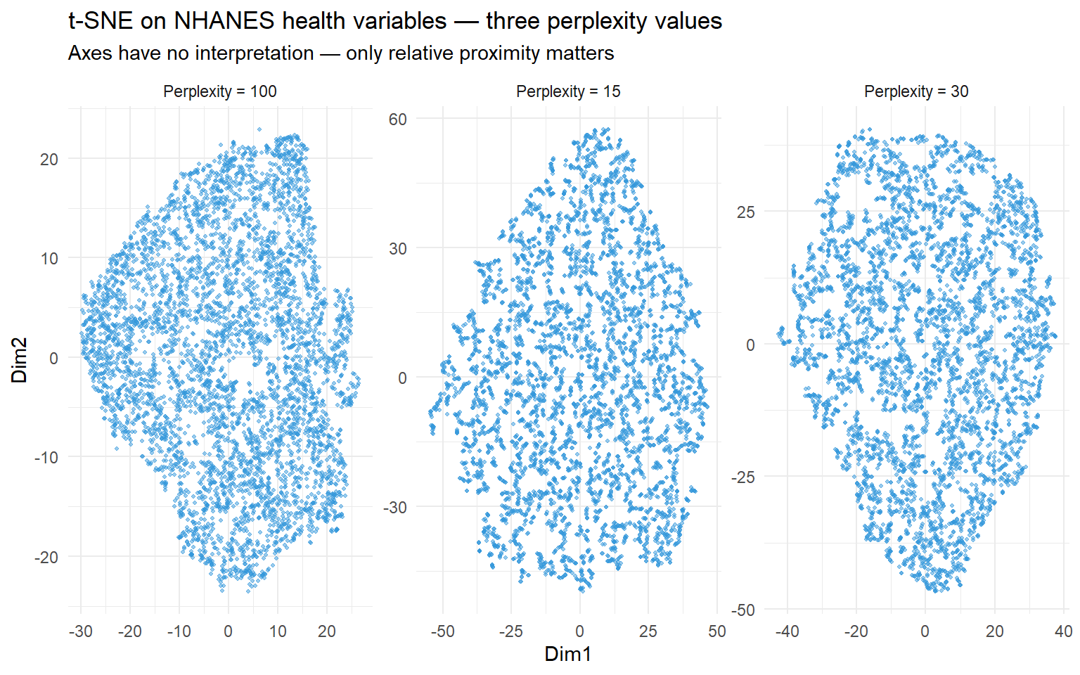

# Compare PCA and t-SNE (perplexity = 30) side by side
pca <- prcomp(X)

df_pca <- data.frame(Dim1 = pca$x[, 1], Dim2 = pca$x[, 2], Method = "PCA")
df_tsne <- data.frame(Dim1 = tsne_30$Y[, 1], Dim2 = tsne_30$Y[, 2], Method = "t-SNE (perplexity = 30)")

df_both <- rbind(df_pca, df_tsne)
df_both$Age <- rep(dat$Age, 2)

ggplot(df_both, aes(Dim1, Dim2, colour = Age)) +
  geom_point(size = 0.8, alpha = 0.6) +
  scale_colour_viridis_c(option = "plasma") +
  facet_wrap(~ Method, scales = "free") +
  labs(title = "PCA vs t-SNE — coloured by Age",
       subtitle = "t-SNE separates the age gradient more clearly in local neighbourhoods") +
  theme_minimal()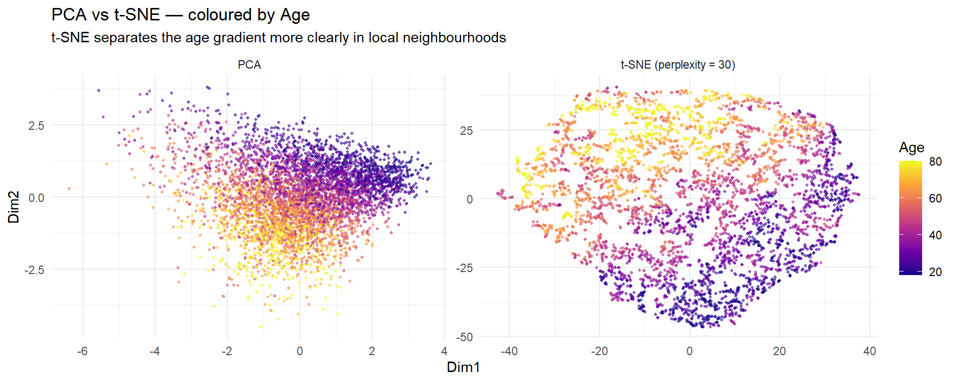

Interpretation: With only five variables, PCA and t-SNE reveal similar structure. The advantage of t-SNE becomes dramatic with hundreds or thousands of variables — as in the scRNA-seq PBMC3k data in Project 3, where t-SNE separates cell types that overlap completely in PCA space.

4 Guided Practice

R is loading in the background — exercises will be interactive once the status bar disappears.

Hints

Rtsne(X, dims = 2, perplexity = 30, check_duplicates = FALSE)$Y gives the 2D coordinates
Use set.seed() before every t-SNE run for reproducibility
Colour by original variables to interpret what drives the t-SNE structure
If the plot looks completely random, try a different perplexity

5 Retrieval Challenge

Model Answer

# K-means on t-SNE coordinates
set.seed(42)
km_tsne <- kmeans(tsne30$Y, centers = 3, nstart = 25)

# K-means on original scaled data
km_orig <- kmeans(X, centers = 3, nstart = 25)

df <- data.frame(
  Dim1 = tsne30$Y[, 1], Dim2 = tsne30$Y[, 2],
  tsne_cluster = factor(km_tsne$cluster),
  orig_cluster = factor(km_orig$cluster)
)

library(tidyr)
df_long <- pivot_longer(df, cols = c(tsne_cluster, orig_cluster),
                        names_to = "method", values_to = "cluster")

ggplot(df_long, aes(Dim1, Dim2, colour = cluster)) +
  geom_point(size = 0.8, alpha = 0.5) +
  facet_wrap(~ method) +
  theme_minimal()

# Cross-tabulation
table(tsne = km_tsne$cluster, original = km_orig$cluster)

Clustering on t-SNE coordinates and on original variables often gives different results because t-SNE emphasises local structure. Clustering on t-SNE is reasonable for exploration but the clusters are defined by the t-SNE geometry, not the original variable space.

6 Why-Questions

Q: “Can I use t-SNE instead of PCA before clustering?”

You can, but be cautious. Clustering on t-SNE coordinates is exploratory and the clusters are defined by the 2D projection, not the original space. Distances in t-SNE are distorted, so k-means on t-SNE will find clusters based on visual proximity in the plot. The standard pipeline for high-dimensional data (like scRNA-seq) is: PCA first to reduce to ~50 components → t-SNE/UMAP on the PC scores for visualisation → cluster in PCA space, not t-SNE space.

Q: “My t-SNE plot looks different every time I run it. Is something wrong?”

No — t-SNE is stochastic. The random initialisation means different runs produce different layouts, though the overall cluster structure should be similar if the perplexity is appropriate. Always use set.seed() for reproducibility. If the gross structure (which groups are separated vs merged) changes between runs, the clusters are not stable and you should increase nstart or try different perplexity values.

Q: “How is t-SNE different from UMAP?”

Both are nonlinear dimensionality reduction methods that preserve local structure. t-SNE minimises KL divergence between probability distributions in high-D and 2D. UMAP uses a different mathematical framework (topological data analysis) that better preserves global structure — distant clusters in the high-D space remain distant in the UMAP plot, which is not guaranteed with t-SNE. UMAP is also faster and produces deterministic results for fixed seeds. In practice, both are used for visualisation; UMAP is now more common in genomics. See the next page for details.