F1 — What is Statistical Learning?

1 Concept: The Learning Problem

1.1 The statistical learning framework

We observe data \((x_1, y_1), \ldots, (x_n, y_n)\) and assume:

\[Y = f(\mathbf{X}) + \varepsilon\]

where \(f\) is the true unknown function we want to estimate, and \(\varepsilon\) is irreducible noise with \(\mathbb{E}[\varepsilon] = 0\).

Statistical learning is the task of estimating \(\hat{f}\) from data, so that:

\[\hat{Y} = \hat{f}(\mathbf{X})\]

gives useful predictions for new observations.

1.2 Two goals: inference vs prediction

Goal	Question	Interpretability needed?
Inference	How does \(X_j\) affect \(Y\)?	Yes — coefficient meaning matters
Prediction	What is \(\hat{Y}\) for new \(X\)?	No — accuracy is the criterion

In STA230, we move toward prediction: we evaluate models by how well they perform on unseen data, not how well they fit the data they were trained on.

1.3 Supervised vs unsupervised

Supervised: we have both \(\mathbf{X}\) and \(Y\). Regression (continuous \(Y\)) or classification (categorical \(Y\)).
Unsupervised: no \(Y\). We look for structure in \(\mathbf{X}\) alone — clusters, principal components.

The course covers all three: supervised regression (Block 1), supervised classification (Block 2), unsupervised methods (Block 3).

1.4 The irreducible error

No matter how good \(\hat{f}\) is, we cannot reduce the prediction error below:

\[\text{Var}(\varepsilon) = \sigma^2_\varepsilon\]

This is the irreducible error — noise inherent in the data generating process. The reducible part is \(\mathbb{E}[(f(\mathbf{X}) - \hat{f}(\mathbf{X}))^2]\), which we can minimise by choosing \(\hat{f}\) well.

2 Quiz

The error caused by choosing the wrong model class

Variance of ε — noise in Y that no model can eliminate, even a perfect f̂

The difference between training error and test error

The error from not having enough training data

The model is Y = f(X) + ε. Even if we recover f exactly (f̂ = f), our predictions still have error Var(ε). This cannot be reduced — it reflects genuine randomness in the outcome. The reducible error E[(f(X) − f̂(X))²] is what better models, more data, or better features can address.

When we want to minimise test MSE on future data

When the goal is inference — understanding how each predictor affects the outcome

When n is very large relative to p

When we use cross-validation for model selection

If the goal is prediction, a black-box model with low test error is fine. If the goal is inference — "does X₂ affect Y after adjusting for X₁?" — we need interpretable models (linear regression, LASSO) where coefficients have clear meaning. In clinical or policy applications, inference often matters as much as prediction accuracy.

Supervised learning uses all available predictors; unsupervised uses only a subset

Supervised methods always require more data

Supervised learning has a response variable Y; unsupervised only has X

Unsupervised methods are always simpler than supervised ones

In supervised learning we use (X, Y) pairs to learn f. In unsupervised learning there is no Y — we search for structure in X alone (clusters, latent dimensions). Unsupervised is harder to evaluate because there is no ground truth to compare predictions against.

3 Worked Example

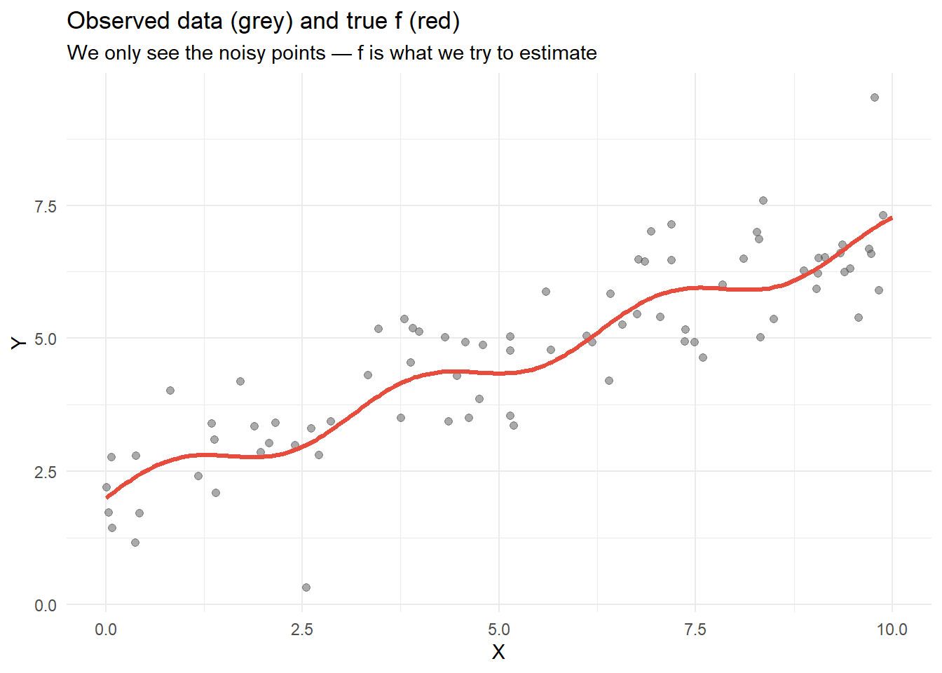
# The true f (we know it because we simulated the data)
# In real life f is unknown — we only see the noisy Y
x_grid <- seq(0, 10, length.out=200)
f_vals <- f_true(x_grid)

ggplot(dat, aes(x, y)) +
  geom_point(alpha=0.5, size=1.8, colour="#555") +
  geom_line(data=data.frame(x=x_grid, y=f_vals),
            aes(x, y), colour="#e74c3c", linewidth=1.2) +
  labs(title="Observed data (grey) and true f (red)",
       subtitle="We only see the noisy points — f is what we try to estimate",
       x="X", y="Y") +
  theme_minimal()

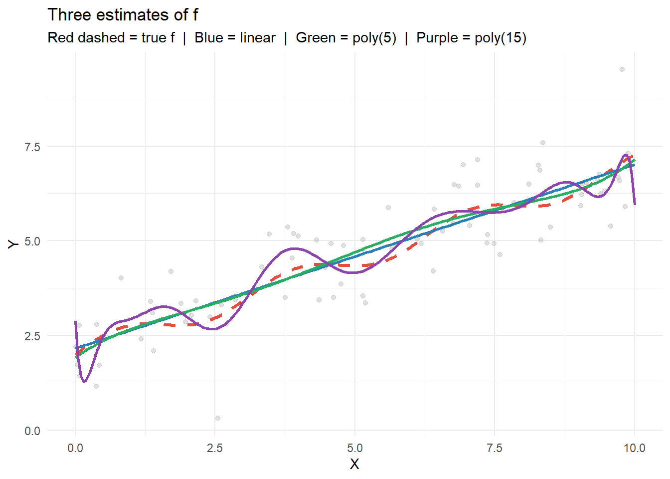
# Three estimates with different complexity
fit_linear <- lm(y ~ x, data=dat)
fit_poly5  <- lm(y ~ poly(x, 5), data=dat)
fit_poly15 <- lm(y ~ poly(x, 15), data=dat)

preds <- data.frame(
  x     = x_grid,
  true  = f_vals,
  linear = predict(fit_linear, newdata=data.frame(x=x_grid)),
  poly5  = predict(fit_poly5,  newdata=data.frame(x=x_grid)),
  poly15 = predict(fit_poly15, newdata=data.frame(x=x_grid))
)

ggplot(dat, aes(x, y)) +
  geom_point(alpha=0.3, size=1.5, colour="#999") +
  geom_line(data=preds, aes(x, true),   colour="#e74c3c", linewidth=1.2, linetype="dashed") +
  geom_line(data=preds, aes(x, linear), colour="#2980b9", linewidth=1)  +
  geom_line(data=preds, aes(x, poly5),  colour="#27ae60", linewidth=1)  +
  geom_line(data=preds, aes(x, poly15), colour="#8e44ad", linewidth=1)  +
  labs(title="Three estimates of f",
       subtitle="Red dashed = true f  |  Blue = linear  |  Green = poly(5)  |  Purple = poly(15)",
       x="X", y="Y") +
  theme_minimal()

4 Guided Practice

R is loading in the background — the exercises below will be interactive once the status bar disappears.

Hints

mean((y_test - predict(fit_l, newdata=data.frame(x=x_test)))^2) for test MSE
The model with the lowest training MSE is not necessarily the best model
This is the core tension of statistical learning — which the next section formalises

5 Retrieval Challenge

Model answers

Q1: \(\sigma^2 = 0.9^2 = 0.81\)

Q2: No. The expected test MSE for any estimator is at least \(\sigma^2 = \text{Var}(\varepsilon)\). Perfect knowledge of \(f\) cannot remove the noise in \(Y\).

Q3: poly(20) will have lower training MSE than poly(15) — more flexibility always reduces training error. But test MSE will likely be higher — the model overfits the training noise.

6 Why-Questions

Q: “We evaluate models on test data. What counts as ‘test data’?”

Test data is any data that was not used to fit the model. This includes: - A held-out portion of your dataset (train/test split) - Future real observations - Data from a different study (external validation)

The key requirement: the model never saw this data during training. If you use test data to make model choices (e.g., selecting which polynomial degree is best), that data is no longer a clean test set — it becomes part of your model selection process.