F2 — Bias-Variance Tradeoff

1 Concept: The Most Important Trade-off in Statistical Learning

1.1 Decomposing prediction error

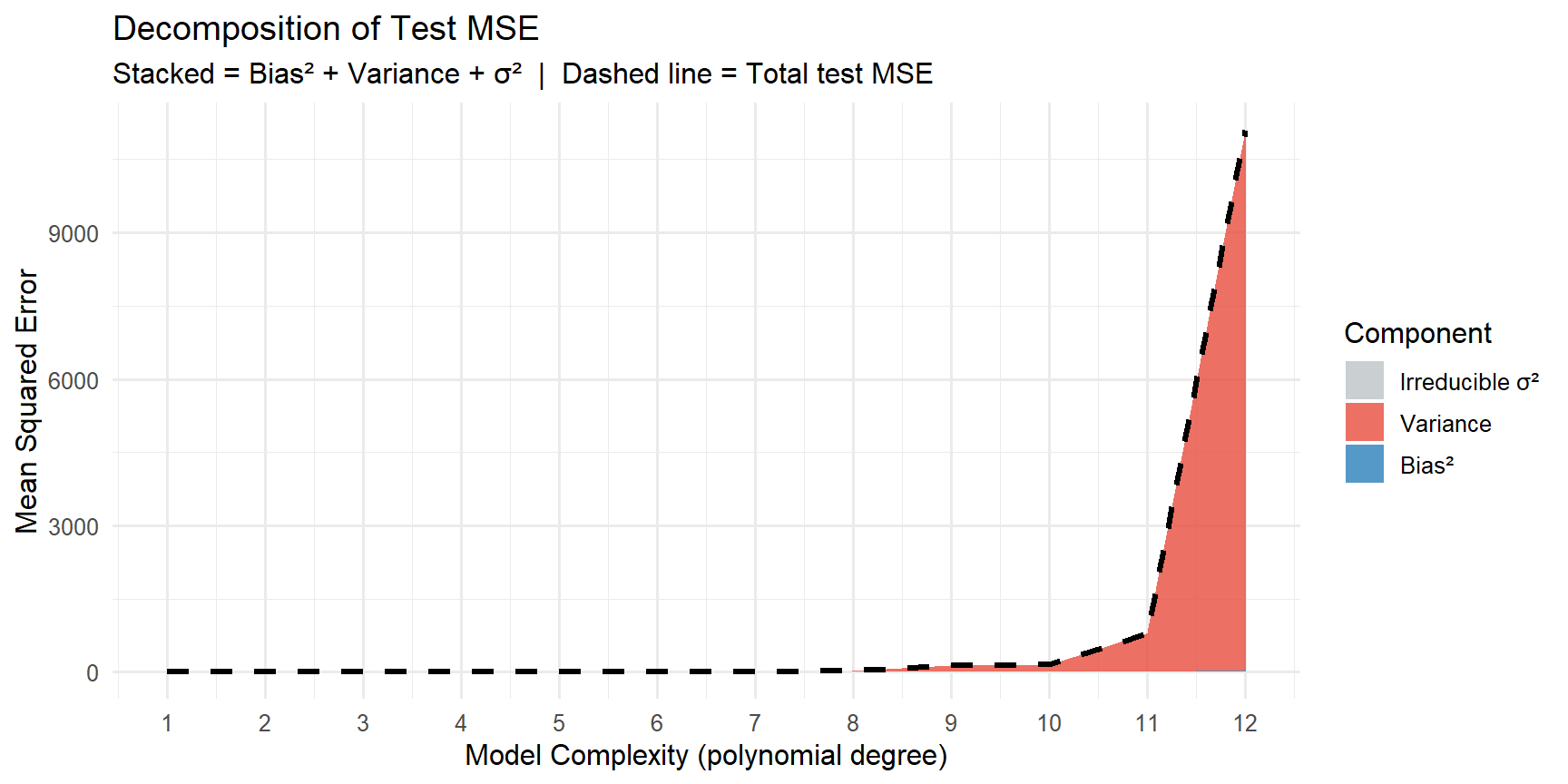
For a fixed test point \(x_0\), the expected test MSE decomposes as:

\[\underbrace{\mathbb{E}\left[(y_0 - \hat{f}(x_0))^2\right]}_{\text{Expected test MSE}} = \underbrace{\left[\text{Bias}(\hat{f}(x_0))\right]^2}_{\text{Bias}^2} + \underbrace{\text{Var}(\hat{f}(x_0))}_{\text{Variance}} + \underbrace{\sigma^2_\varepsilon}_{\text{Irreducible}}\]

where the expectation is over repeated training sets.

Component	Definition	Changes with complexity?
Bias²	How far \(\mathbb{E}[\hat{f}(x_0)]\) is from \(f(x_0)\)	Decreases as complexity increases
Variance	How much \(\hat{f}(x_0)\) varies across training sets	Increases as complexity increases
Irreducible	\(\sigma^2_\varepsilon\) — noise floor	Fixed, never changes

1.2 The U-shaped test error curve (ESL Figure 7.1)

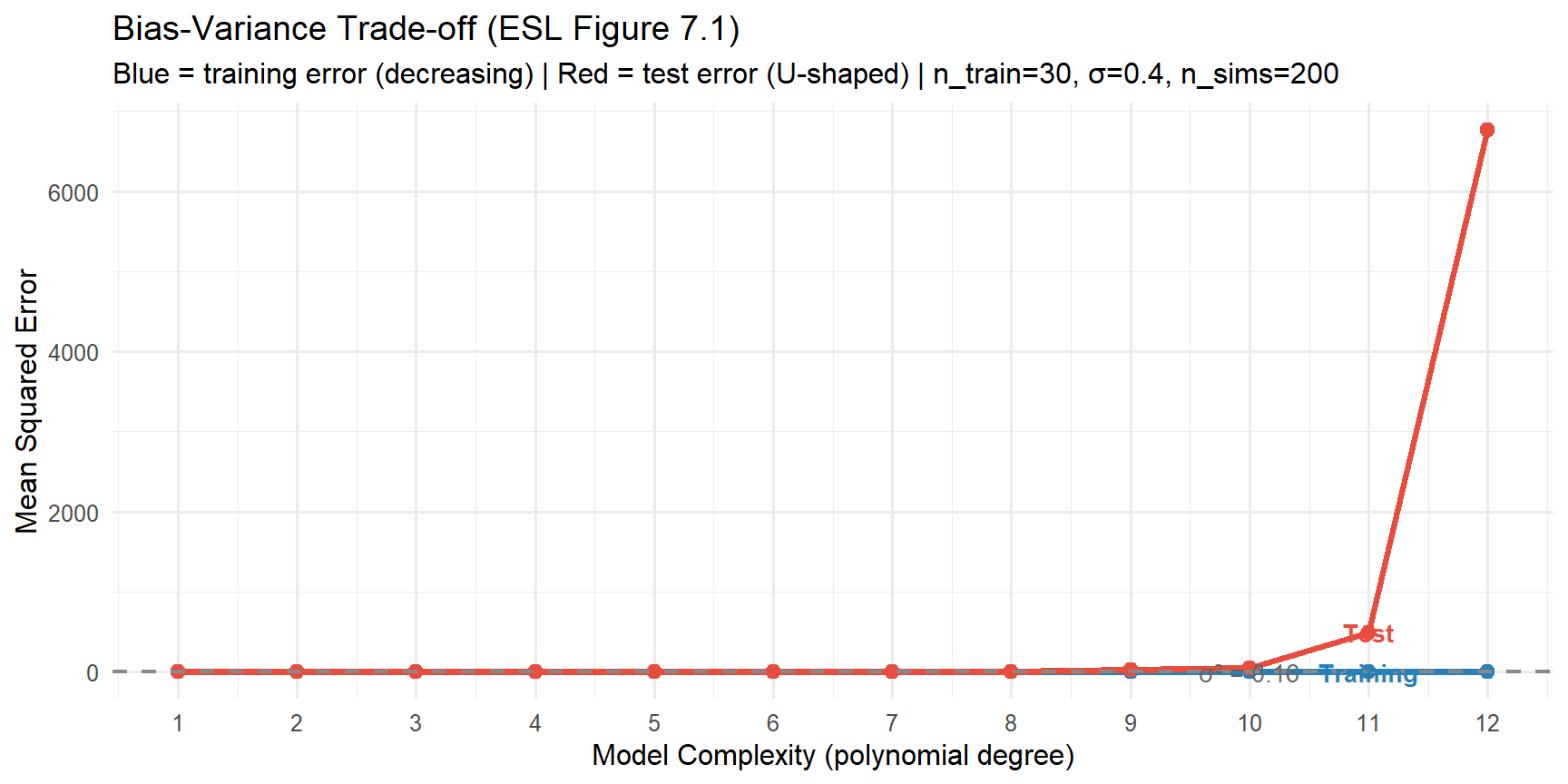
This is the central figure of the course:

Training error (blue): monotonically decreasing — more complex models always fit the training data better
Test error (red): U-shaped — first decreases as we reduce bias, then increases as variance dominates
The minimum of the test error curve is the sweet spot: not too simple, not too complex

Key message

A model that fits the training data perfectly is not necessarily a good model. The goal is to generalise to new data — and that requires balancing bias against variance.

1.3 Two approaches to finding the sweet spot

Analytical — penalise model complexity in the selection criterion (AIC, BIC, adjusted R²)
Data-driven (resampling) — directly estimate test error from data (cross-validation, train/test split)

Block 1 uses both. Cross-validation is covered in F5.

2 Quiz

Both bias and variance increase

Bias increases, variance decreases

Bias decreases, variance increases

Both bias and variance decrease

A simple model (e.g. linear) may be too rigid to capture the true f — it has high bias but low variance (similar fit across training sets). A complex model (e.g. poly(20)) can capture f closely but is sensitive to which training data it saw — it has low bias but high variance. This is the fundamental trade-off.

High bias — the model is too simple

High variance — the model is overfitting the training data

High irreducible error — the noise level is too large

The test set is too small to give a reliable estimate

A very low training error paired with a much higher test error is the classic signature of overfitting (high variance). The model memorised the training data, including its noise, rather than learning the underlying pattern f. The large train-test gap is the diagnostic.

Bias²

Variance

Irreducible error σ²ε

All three can be reduced with enough data

Irreducible error σ²ε is the variance of ε — noise inherent in the data-generating process. Even if f̂ = f exactly, predictions still have error Var(ε). Bias² → 0 as the model becomes flexible enough to approximate f. Variance → 0 with infinite training data. But σ²ε is fixed by nature.

3 Worked Example: Reproducing ESL Figure 7.1

The code below simulates many training sets, fits polynomial models of increasing degree, and plots training error vs test error vs complexity — reproducing the key figure from Hastie, Tibshirani & Friedman (2009).

set.seed(42)
sigma_eps <- 0.4     # true noise SD
n_sims    <- 200     # number of training sets
n_train   <- 30
n_test    <- 500
degrees   <- 1:12

# Fixed test set (large, to get accurate estimate of test error)
x_test <- seq(0, 1, length.out=n_test)
y_test <- f_true(x_test) + rnorm(n_test, 0, sigma_eps)

results <- lapply(degrees, function(d) {
  train_errs <- test_errs <- numeric(n_sims)
  for (i in seq_len(n_sims)) {
    # New training set each simulation
    x_tr <- sort(runif(n_train, 0, 1))
    y_tr <- f_true(x_tr) + rnorm(n_train, 0, sigma_eps)
    fit  <- lm(y_tr ~ poly(x_tr, d))
    # Training MSE
    train_errs[i] <- mean(residuals(fit)^2)
    # Test MSE on fixed test set
    x_poly <- poly(x_test, d, coefs=attr(poly(x_tr, d), "coefs"))
    test_errs[i]  <- mean((y_test - cbind(1, x_poly) %*% coef(fit))^2)
  }
  data.frame(degree=d,
             train_mse = mean(train_errs),
             test_mse  = mean(test_errs))
})
res <- do.call(rbind, results)

# Add irreducible error baseline
irred <- sigma_eps^2

# Plot: training vs test error
ggplot(res, aes(x=degree)) +
  geom_line(aes(y=train_mse), colour="#2980b9", linewidth=1.4) +
  geom_point(aes(y=train_mse), colour="#2980b9", size=2.5) +
  geom_line(aes(y=test_mse), colour="#e74c3c", linewidth=1.4) +
  geom_point(aes(y=test_mse), colour="#e74c3c", size=2.5) +
  geom_hline(yintercept=irred, linetype="dashed", colour="#888", linewidth=0.8) +
  annotate("text", x=10, y=irred+0.01, label=paste0("σ² = ", irred),
           colour="#666", size=3.5) +
  annotate("text", x=11, y=res$train_mse[11]+0.03, label="Training",
           colour="#2980b9", size=3.5, fontface="bold") +
  annotate("text", x=11, y=res$test_mse[11]+0.03, label="Test",
           colour="#e74c3c", size=3.5, fontface="bold") +
  scale_x_continuous(breaks=degrees) +
  labs(title="Bias-Variance Trade-off (ESL Figure 7.1)",
       subtitle=paste0("Blue = training error (decreasing) | Red = test error (U-shaped) | ",
                       "n_train=", n_train, ", σ=", sigma_eps, ", n_sims=", n_sims),
       x="Model Complexity (polynomial degree)",
       y="Mean Squared Error") +
  theme_minimal(base_size=12)

# Show all three components: Bias², Variance, Irreducible
set.seed(42)
bv_decomp <- lapply(degrees, function(d) {
  preds_mat <- matrix(NA, nrow=n_sims, ncol=n_test)
  for (i in seq_len(n_sims)) {
    x_tr <- sort(runif(n_train, 0, 1))
    y_tr <- f_true(x_tr) + rnorm(n_train, 0, sigma_eps)
    fit  <- lm(y_tr ~ poly(x_tr, d))
    x_poly <- poly(x_test, d, coefs=attr(poly(x_tr, d), "coefs"))
    preds_mat[i, ] <- cbind(1, x_poly) %*% coef(fit)
  }
  mean_pred <- colMeans(preds_mat)
  bias2     <- mean((mean_pred - f_true(x_test))^2)
  variance  <- mean(apply(preds_mat, 2, var))
  data.frame(degree=d, bias2=bias2, variance=variance, irreducible=irred,
             test_mse=bias2+variance+irred)
})
bv <- do.call(rbind, bv_decomp)

bv_long <- tidyr::pivot_longer(bv, c(bias2, variance, irreducible),
                                names_to="component", values_to="mse")
bv_long$component <- factor(bv_long$component,
                             levels=c("irreducible","variance","bias2"),
                             labels=c("Irreducible σ²","Variance","Bias²"))

ggplot(bv_long, aes(x=degree, y=mse, fill=component)) +
  geom_area(alpha=0.8, position="stack") +
  geom_line(data=bv, aes(x=degree, y=test_mse), inherit.aes=FALSE,
            colour="black", linewidth=1.2, linetype="dashed") +
  scale_fill_manual(values=c("Irreducible σ²"="#bdc3c7",
                              "Variance"="#e74c3c",
                              "Bias²"="#2980b9")) +
  scale_x_continuous(breaks=degrees) +
  labs(title="Decomposition of Test MSE",
       subtitle="Stacked = Bias² + Variance + σ²  |  Dashed line = Total test MSE",
       x="Model Complexity (polynomial degree)",
       y="Mean Squared Error",
       fill="Component") +
  theme_minimal(base_size=12)

4 Interactive Exploration: Build the Figure Yourself

R is loading in the background — the exercises below will be interactive once the status bar disappears.

The blocks below let you change parameters and immediately see how the bias-variance curve changes. Run each block, then modify the parameters to compare different settings.

What to try

More data (n_train = 100): Does the U-shape shift right? Why? More data reduces variance → higher complexity becomes viable.
More noise (sigma_eps = 0.8): Does the test error floor rise? Does the optimal degree change? Higher σ² raises the irreducible floor. The bias-variance tradeoff shape stays the same.
Less noise (sigma_eps = 0.1): Can you get a test error close to the irreducible floor? With low noise a flexible model can nearly recover f perfectly.
Small training set (n_train = 15): Does the optimal degree drop? Why? Small n → high variance for complex models → simple models preferred.

5 Guided Practice: Fitting multiple degrees side by side

The next blocks fit degree 1, 3, 6, and 12 models to the same training data and plot them together so you can see the fit directly.

Tasks

TASK 1: Which degree has the lowest training MSE? Is that the best model?
TASK 2: Which degree is closest to the irreducible error floor on the test set?
TASK 3: Change set.seed(7) to set.seed(123) and re-run both blocks. Does the ranking change? What does this tell you about variance?
TASK 4: The degree-12 fit looks very wiggly. What would happen to its test MSE with 300 training observations instead of 30?

6 Retrieval Challenge

Model answers

Q1: \(0.02 + 0.15 + 0.16 = 0.33\)

Q2: Variance decreases. More training data makes \(\hat{f}\) more stable across samples.

Q3: Bias² increases. A simpler model cannot approximate \(f\) as closely.

Q4: \(0.16 / 0.33 \approx 0.485\) — nearly half the test error is irreducible.

7 Why-Questions

Q: “If I average many complex models, does that help?”

Yes — this is the idea behind ensemble methods (Random Forests, Boosting). Averaging reduces variance without increasing bias much. A single poly(12) model has high variance. The average of 500 independently trained poly(12) models has nearly zero variance (the averages converge to \(\mathbb{E}[\hat{f}]\)). Bagging exploits exactly this property.

Q: “My training error is 0.01. Is my model good?”

Training error alone tells you almost nothing. You need the test error to know if the model generalises. A training error of 0.01 is consistent with either: (a) a great model that approximates \(f\) well, or (b) severe overfitting where the model memorised the training data. Only the test error distinguishes these.